Understanding Markov Chains with the Black Friday Puzzle
This week we celebrate Thanksgiving and Black Friday with a fun puzzle and our first look at Markov Chains!
In the United States, Black Friday is a Dionysian ritual celebrated immediately after Thanksgiving. Having exhausted the limits of the physical consumption of food the day before, frenzied shoppers crowd into busy stores and ritualistically explore the higher forces of consumerism. Devoid of reason, this bizarre experience can only be understood using the tools of Probability Theory!

Can probability save us from our madness?
The Black Friday Puzzle
You are the Senior Data Scientist for Bayes Books, a very successful chain of nearly identical bookstores. Living in a post-Amazon age, Bayes Books has diversified their collection and organized their stores into 5 main sections: Books, Children's Books, Puzzles, Toys, and Music. The most important problem for the store is optimizing the number of Sales Associates in each section. Past research has shown that 1 employee for every 100 customers in a section is the ideal amount to minimize salary cost and optimize sales.
Under normal circumstances customers flow through the store in a very predictable pattern, given the average number of customers it is easy to figure out how many Sales Associates to put in each section. But on Black Friday all that changes! The customers, consumed with a mystic passion for reduced prices behave in very hard to understand patterns, jumping from section to section erratically!
Your responsibility is to determine the ideal number of Sales Associates per section. Immediately you task your Junior Data Scientists with compiling data from past Black Fridays in an attempt to solve this problem. The good news is they developed a deep learning algorithm to predict the total number of customers in the store a given time. Unfortunately, the rest of the analysis looks grim; customers seem to move from section to section at random! Sometimes they will remain in Books for 20 minutes then all of a sudden rush across the store to Music, only to run back to Books a minute later!
The only thing that the Junior Data Scientists can give you is the probability that each customer moves to a given section each minute. For example:
If a customer is in Books, there's a 50% chance they'll stay there, a 20% chance they'll go to Children's Books, a 15% they'll move to Puzzles, 10% chance they'll move to Toys and a 5% chance they'll move to Music.
We can visualize this as a graph of customer movement.
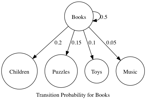
Given that you are in the Books section, where will you be next?
Of course this is just the data for Books, if we take all the data we get

The full Markov Chain representation of our problem
Yikes! The only thing this image helps with is letting us know that this is a pretty crazy problem! We can represent this data is a much easier by putting it in a table.

Transition graph in table form
This view helps a bit, but this still seems like a tricky problem to solve.
Markov Chains
The problem we've outlined so far is formally called a Markov Chain. The key things that make this a Markov Chain are that each person transitions from each state probabilistically and the only state that matters is where the person currently is. Normally there might be a relationship between starting in Books, moving to Children's Books and then going to Toys. Because of the Black Friday frenzy customers move only based on where they currently are, running back and forth across the store multiple times is a possible behavior.
To put it more poetically: In a Markov Chain the future is uncertain, and all that matters for tomorrow is where you are today.
Expected Number of Sales Associates
Just like the Toy Collectors Problem in the last post, we're facing a question about Expectation. We want to know how many Sales Associates to put in each area. As always when dealing with a hard probability problem it's always best to start with a simplification; study how it behaves and add complexity from there.
Let's say there are 100 people in Books right now (and nobody anywhere else). We're assuming that our movements are all happening in 1-minute chunks. That is with the tick of each minute people move based on the table above. To keep this simple, we only care about the expected people in Books. We'll use \(n_{books\_t}\) for the number of people in books at time \(t\) and \(p_{x\rightarrow books}\) for the probability of transitions from \(x\) to Books.
For our first time step all we care about is how many people are expected to stay in Books
$$E[n_{books\_1}] = p_{books\rightarrow books}\cdot n_{books\_ 0} = 0.5 \cdot 100 = 50$$
That was easy, but as soon as we take our next step it gets much more complicated. Now we have to consider how many people are going to come back to Books from other states!
$$E[n_{books\_2}] = p_{books\rightarrow books}\cdot n_{books\_ 1} + p_{children\rightarrow books}\cdot n_{children\_ 1} + p_{puzzles\rightarrow books}\cdot n_{puzzles\_ 1} ...$$
If you had some free time you could feasibly calculate that by hand, but step 3 is even worse that that! For step 3 we additionally have to recalculate the populations of each area of the store which is an identical process to the one for Books!
Linear Algebra to the Rescue!
If you remember your Linear Algebra this pattern should look very familiar (and if you don't remember or never learned, prepare to be motivated!). This pattern of calculation is exactly how Matrix Multiplication works! Specifically it would be the dot product of our Transition Matrix (i.e. the table we made) and a vector of our initial populations. To make this a bit more clear, we can represent our table of Transition Probabilities as a Matrix:
$$\begin{bmatrix} 0.5 & 0.1 & 0.1 & 0.05 & 0.2\\ 0.2 & 0.3 & 0.2 & 0.15 & 0.1 \\ 0.15 & 0.2 & 0.3 & 0.3 & 0.1 \\ 0.1 & 0.3 & 0.2 & 0.4 & 0.1 \\ 0.05 & 0.1 & 0.2 & 0.1 &0.5 \end{bmatrix}$$
This is just converting our labeled states into indices in a matrix. Books is now column 1 and Music column 5, the transition probability for Books to Music is the value a column 1 and row 5.
Now we can represent our initial populations a Vector of 5 values, reach value representing the population in a given state. Our simple model of 100 people in Books looks like this:
$$\begin{bmatrix} 100\\ 0 \\ 0 \\ 0 \\ 0\end{bmatrix}$$
We calculate step 1 from before by taking the dot product of the Transition Matrix with our Vector representing our population at \(t=0\)
$$\left[ \begin{array}{ccccc} 0.5 & 0.1 & 0.1 & 0.05 & 0.2\\ 0.2 & 0.3 & 0.2 & 0.15 & 0.1 \\ 0.15 & 0.2 & 0.3 & 0.3 & 0.1 \\ 0.1 & 0.3 & 0.2 & 0.4 & 0.1 \\ 0.05 & 0.1 & 0.2 & 0.1 &0.5 \end{array} \right] \cdot \left[ \begin{array}{c} 100\\ 0\\ 0\\ 0\\ 0\\ \end{array} \right] = \left[ \begin{array}{c} 50\\ 20\\ 15\\ 10\\ 5\\ \end{array} \right] $$
That was pretty easy, and now we also have the population for all other states. To calculate step 2 we simply replace our original population vector with the new one:
$$\left[ \begin{array}{ccccc} 0.5 & 0.1 & 0.1 & 0.05 & 0.2\\ 0.2 & 0.3 & 0.2 & 0.15 & 0.1 \\ 0.15 & 0.2 & 0.3 & 0.3 & 0.1 \\ 0.1 & 0.3 & 0.2 & 0.4 & 0.1 \\ 0.05 & 0.1 & 0.2 & 0.1 &0.5\end{array} \right] \cdot \left[ \begin{array}{c} 50\\ 20\\ 15\\ 10\\ 5\\ \end{array} \right] = \left[ \begin{array}{c} 30.0 \\ 21.0 \\ 19.5 \\ 18.5 \\ 11.0 \\ \end{array} \right] $$
And of course, step 3, which would have taken most of an evening to calculate by hand, is just the same thing repeated!
$$\left[ \begin{array}{ccccc} 0.5 & 0.1 & 0.1 & 0.05 & 0.2\\ 0.2 & 0.3 & 0.2 & 0.15 & 0.1 \\ 0.15 & 0.2 & 0.3 & 0.3 & 0.1 \\ 0.1 & 0.3 & 0.2 & 0.4 & 0.1 \\ 0.05 & 0.1 & 0.2 & 0.1 &0.5 \end{array} \right] \cdot \left[ \begin{array}{c} 30.0 \\ 21.0 \\ 19.5 \\ 18.5 \\ 11.0 \\ \end{array} \right] = \left[ \begin{array}{c} 22.175\\ 20.075\\ 21.200\\ 21.700\\ 14.850\\ \end{array} \right] $$
The Stationary Distribution!
What happens if we keep on doing this? After 30 steps of this process here is our population vector:
$$\begin{bmatrix}17.90006\\ 18.86964\\ 21.67067\\ 22.77285\\ 18.78677\end{bmatrix}$$
And then after 1,000 steps:
$$\begin{bmatrix}17.90006\\ 18.86964\\ 21.67067\\ 22.77285\\ 18.78677\end{bmatrix}$$
Remarkable! They're identical! What if we started with a different initial population:
$$\left[ \begin{array}{c} 0\\ 0 \\ 0\\ 0\\ 100\\ \end{array} \right] \text{repeat 1000x} \left[ \begin{array}{c} 17.90006\\ 18.86964\\ 21.67067\\ 22.77285\\ 18.78677\\ \end{array} \right]$$
It's still the same! The remarkable thing about Markov Chains is, as long as you can get to any state from any state in a finite number of steps, the distribution of the population in each state remains the same. This is referred to as the Stationary Distribution of a Markov Chain.
Putting our Answer Together
Your team of Junior Data Scientists has put a bunch of data in a Deep Neural Net and determined that for a particular store there should be a pretty stable population of 6,000 people throughout Black Friday. If we look at our stable distribution as a percentage of the whole population we can just perform scalar multiplication and get our answer:
$$6,000 \cdot \left[ \begin{array} {c} 0.1790006\\ 0.1886964\\ 0.2167067\\ 0.2277285\\ 0.1878677\\ \end{array} \right]=\left[ \begin{array} {c} 1074.003\\ 1132.179\\ 1300.240\\ 1366.371\\ 1127.206\\ \end{array} \right]$$
Given that we need 1 Sales Associate per 100 customers, rounding our answers, we should have 11 Sales Associates in Books, 11 in Children's, 13 in Puzzels, 14 in Toys and 11 in Music. Given the complexity we started with its amazing that just a little Linear Algebra gives us pretty quick and clear answer!
But wait there's more!
It's amazing how much Linear Algebra has been able to help us solve our problem! But there's something even more incredible. We can break down Square Matrices into something called Eigenvectors and Eigenvalues. Without getting into too much detail, Eigenvectors represent central tendencies of the data in a Square Matrix, and Eigenvalues weight those tendencies. So the Eigenvector corresponding to the largest Eigenvalue represents the strongest summary of the data.
Any software package that can handle Linear Algebra can calculate the Eigenvectors and Eigenvalues for a square matrix. Here is the R code to do it:
#our transition matrix
A = matrix(c(0.5,0.1,0.1,0.05,0.2,
 0.2, 0.3, 0.2,0.15 , 0.1,
 0.15,0.2 , 0.3, 0.3,0.1,
 0.1 ,0.3 , 0.2 , 0.4 ,0.1,
 0.05 , 0.1 , 0.2 , 0.1,0.5),nrow=5,ncol=5,byrow=1)

#we just want the Eigenvectors
eigenvectors <- eigen(A)$vectors
The Eigenvectors are sorted by by their Eigenvalues. Our first Eigenvector is:
$$\begin{bmatrix}0.3985040\\ 0.4200896\\ 0.4824481\\ 0.5069856\\ 0.4182447\\ \end{bmatrix}$$
Not particularly interesting at first but if we clean it up a little bit...
first_ev <- eigenvectors[,1]
#normalize this
first_ev <- first_ev/sum(first_ev)
We end up with a very familiar Vector!
$$\begin{bmatrix}0.1790006\\ 0.1886964\\ 0.2167067\\ 0.2277285\\ 0.1878677\\ \end{bmatrix}$$
The principle Eigenvector of the Transition Matrix of a Markov Chain is proportional to the Markov Chain's stationary distribution! That to me is truly amazing.
It is worth noting that in practice, for large Markov Chains, calculating the Eigenvectors is much, much more costly than simply iteratively finding the stationary distribution. So in practice this is less useful. Pragmatics aside, this is truly a remarkable fact!
Conclusion
The Black Friday Puzzle is just one type of Markov Chain. The essential property that made our analysis possible is that given that you are in a state you can always get back to another. In our particular example, you can go from any state directly to any other state, this is not necessary for there to be a stationary distribution. All that is necessary for a stationary distribution is that you can eventually get from state A to state B, for example if you had to go through Toys to get to Books from Puzzles our solution would still work. Of course, it's easy to imagine a Markov Chain with states you can't get back too, and states you can never leave. The latter of these is called an Absorbing Markov Chain and is one of the ways we can solve The Toy Collectors Puzzle from the last post.
If you enjoyed this post please subscribe to keep up to date and follow @willkurt!