Elegance and robustness always seem at odds. In the previous post on the Fundamental Theorem of Calculus we built up an understanding of how and why one of the most beautiful theorems in mathematics allows us to calculate the Integral of a function by using its Antiderivative. This Theorem wonderfully ties together the Calculus of Derivatives with the Calculus of Integrals. Unfortunately finding a way to break this rule is trivially easy!

Absolutely Ridiculous!

If you study math, science or engineering enough you'll find that one of the most useful functions from High school seems oddly absent in places where it seems most useful: the Absolute Value Function. You may have observed that just about anytime you want to use a value that can take both negative and positive values, but you only care about its general magnitude you almost always Square that value rather than take its absolute value. This even comes up in probability, in all my discussion of "Why is Variance $x^2$" I actually never touched on why in the world would we choose $x^2$ rather than the much more intuitive $|x|$. The reason is that the Absolute Value function, while very simple to understand and reason about, has one really big problem: it has no derivative!

To understand why this is we can look at the difference between $x^2$ and $|x|$ when we plot them out.

The problem is in the difference between the sharp point in $|x|$ and the curve in $x^2$. Remember that the derivative is essentially just taking the slope of a very, very tiny piece of the line. With $x^2$ we can visually intuit that as we get a smaller and smaller piece of the line that slope is going to converge. But for $|x|$ that convergence irritatingly never happens right around 0. No matter how far you zoom in there's always going to be that sharp point, and it's never going to look 'smooth'. Real Analysis provides a much fancier description of this problem but the key insight here is that because of that one annoying place in the line we can't take its derivative. What makes this particularly annoying is that everywhere else but around 0 $|x|$ is straight so its slope, and thus the derivative, is easy to calculate.

This not having a Derivative also entails that the Absolute Function does not have an Antiderivative!

No Antiderivate means the Fundamental Theorem of Calculus does us no good!

Easiest Integral!

The really annoying thing is that calculating the Integral for $|x|$ is so easy that nearly anyone can solve it with High school math, even if they never touched Calculus. One of the most basic (and useful) definitions of the Integral is "Area under the curve". If we visualize these areas the the problem is trivial. Here is a visual example using $\int_{0}^{2} |x|$ to help you see:

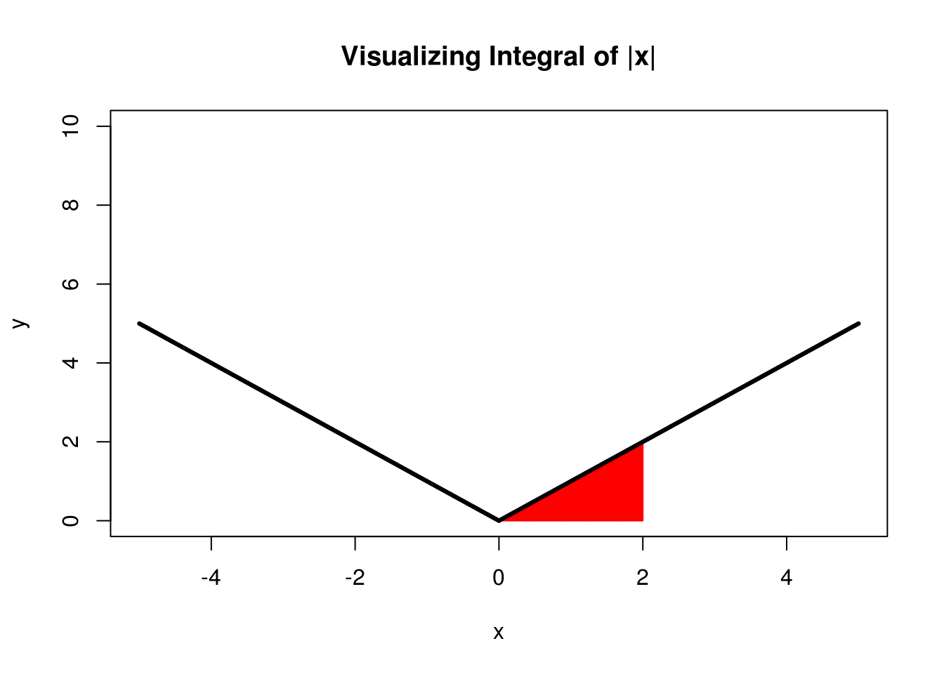
This Integral is simply the Area of a right triangle formed where the line of the function intersects 0! We learn in Highschool geometry that this value is simply $\frac{1}{2}\text{width}\cdot \text{height}$. In this above case $\text{width} = 2 $ and $\text{height} = |2| $. In this case clearly $\int_{0}^{2} |x| = 2$. Part of the simplicity of this is of course that we're starting with 0 but any possible Integral of the Absolute Value function is easy to solve just by adding and substracting triangles.

For example for $\int_{2}^{4} |x|$

We just subtract the missing area from 0-2 (blue) from the total triangle formed by 0-4 (red+blue). Integrals that include a negative value such as $\int_{-2}^{2} |x|$ Are even easier:

We just add the blue and red areas together!

Generalized Area Under the Curve

When finding a more robust way to define the Integral we need to not only be able to solve this problem of Absolute Values, but also still be able to solve all of our old problems. It would be completely useless to come up with a special "Absolute Value Integration" that was unable to also solve the Integral for $x^2$. To make our idea of the Integral more robust we're going to develop a new definition not based on the Fundamental Theorem of Calculus, but rely on this notion of the Area Under the Curve that works so well for the Absolute Value Function.

It turns out that the solution to this problem is fairly obvious if you think about it computationally. From the post on the Fundamental Theorem of Calculus we went over a method of approximating the Integral using discrete sums. For example for $\int_{-2}{4} x^2$ we can use the following code to approximate this integral:

f <- function(x) x^2
dx <- 0.1
xs <- seq(-2,4,by=dx)
approx.int = sum(f(xs))*dx

For our approximate integral we get 25.01 and we know that the exact integral can be computed using the Antiderivative $\frac{1}{3}x^3$ giving us:$$\int_{-2}^{4} x^2 = \frac{1}{3}4^3 - \frac{1}{3}-2^3 = 24$$So our approximation is very close and as we shrink dx it will get closer (e.g. changing dx form 0.1 to 0.01 brings out result to 24.1).

If we visualize this computation we realize that we are using a technique that is very similiar to the one we used to compute the Integral for the Absolute Value Function.

Because we don't have clear cut triangles, we end up building a bunch of little "towers" that approximate the exact area under the curve. As we shrink the size of these towers we'll get better results:

Now what happens if we apply this more general method of calculating the area under the curve to our Absolute Value Function:

f <- function(x) abs(x)
dx <- 0.1
xs <- seq(-2,4,by=dx)
approx.int = sum(f(xs))*dx

We get 10.3 for our approximation and know that the actual Integral from -2 to 4 is: 10. Pretty good! We can also visualize what's happening in the same way we did for $x^2$.

Riemann Integral: Not as Elegant, Much More Intuitive

Here is the general idea of our new method of integration: We divide up the function into a bunch of little towers. As we shrink the size of the towers infinitely small the approximate area calculated by their sum is the Integral. This is the basic idea of what is referred to as the Riemann Integral. In an age of ubiquitous computing, this method of calculating the Integral will naturally arise as a solution to the problem of calculating the area under the curve.

It is important to realize that the Riemann Integral is not just a technique for computing the value of an Integral but allows for a more robust definition of which functions are and are not Integrable. As we dive deeper into mathematics computing numeric solutions decreases in importance but being able to rigorously describe solutions becomes the heart of problem-solving. There are certain concepts in Rigorous Probability with Measure Theory that essentially cannot be computed because they require uncountably infinite sets, but nonetheless they provide much insight into how we think about probability.

Rigorous View of the Riemann Integral

Speaking of rigor, the "many little towers" definition of the Riemann Integral is not exactly its rigorous definition. To arrive at its rigorous definition, we have to realize that when we approximate the area with towers there's really two ways we can think of our tower existing. The first is the tower that is formed above at the maximum of our function in the range dx and the other is the one formed at the minimum in the same. These are technically called the "Supremum" (typically abreviated Sup) and "Infimum" (typically abreviated Inf). These two possibilities are visualized here for a small piece of the Sine function:

If we choose either the Sup or the Inf we can see that there is a certain area of the curve unaccounted for. For the Sup it is the area between the blue line and the curve and for the Inf it is the area between the red line and the curve. Depending on the shape of the function, either the Sup or the Inf for a given tower width will initially be larger assuming we're taking a fairly large dx. The formal, rigorous definition of the Riemann Integral says that a function is Riemann Integrable if (and only if!) the difference between the area of the Inf and Sup approaches 0 as the width of the tower (dx) shrinks.

This may seem like a nitpick, but that's essentially what all of rigorous mathematics is. We want to speak extremely precisely about what everything means so we can avoid large errors in reasoning that result as the accumulation of many small, poorly specified definitions of terms. The view of the Riemann Integral I've presented here is really just glossing over a truly in-depth description of the Riemann Integral you would cover in Real Analysis.

What would a function look like that violates this rule? Imagine a function that as you took smaller and smaller pieces the difference between these two areas never converged. At this point it might be hard to imagine such a function but it turns out some very important examples of functions that do violate this rule come up as we delve deeper into Probability Theory.

Welcome to Integration Theory!

One of the most exciting things about math, that is usually not obvious when we first study it, is how the more rigorous we get the more creative we need to become! Most students having spent just a little time with the Fundamental Theorem of Calculus might believe (or maybe hope) that this is the end of Calculus, but it turns out it is just the beginning!

There is much, much more that could be said about the Riemann Integral. If you find the details of this fascinating and aren't already familiar with the area you'll want to read up on Real Analysis. My personal favorite book, especially for self-study, is Understanding Real Analysis by Stephen Abbott.

As functions get weirder we'd still like to be about to talk about their Integrals, especially in Probability where the Integral is the basis for how we talk about different probabilities. It turns out that as we try to be more rigorous about Probability we also end up quickly running into territory where the Riemann Integral also breaks for us. Before we can go there we're going to have to have a few posts expanding on how we think about more rigorously Probability Theory.

If you enjoyed this post please subscribe to keep up to date and follow @willkurt!