Modern Portfolio Theory and Optimization with JAX

In this post we're going to take a deep dive into understanding Modern Portfolio Theory, a strategy for optimizing assets in an investment portfolio to balance the rate of risk and reward. We'll be solving this optimization problem using JAX and differentiable programming.

In order to understand Modern Portfolio Theory (MPT), we'll start by exploring how we can model a single stock's price movements as cumulative samples from a normal distribution, then we'll extend this model to include multiple, partially correlated stock prices as cumulative samples from a multivariate normal. Then we can see that portfolio optimization boils down to finding the correct weighting of a multivariate normal to both maximize our expected returns while minimizing the variance of these returns.

Modeling Stock Price Movements

Even though MPT can be used to optimize a portfolio for a variety of possible assets, we're going to stick with stock prices. We're going to look at the following 12 Stock prices over the last 120 days.

tickers = ['BRZE','AAPL','SBUX','AAL','WMT','AMZN',
           'TMDX','XOM','NFLX','COIN','VTNR','SIGA']
end_date = date.today() - timedelta(days=1)
start_date = end_date - timedelta(days=120)

Here we can see what our data looks like for the first 5 days:

What our stock price time series data looks like.

Before moving on, we need to start transforming our data so that we can better model it.

Looking at log returns

People new to thinking about stock price movements will typically look at the price history for a particular ticker, focusing on the value of the stock at closing each day.

Here is a quick plot of what this data looks like visualized this way.

Typically when we look at stocks we consider the daily prices over a period of time.

While this may be a common way of thinking about stocks, it's not particularly great mathematically. One problem we can immediately see in this chart is that all of our stocks are at very different scales.

A very common transformation is to look at the log returns for our data, which we can generate with the code below:

ret_data = np.log(stock_data/stock_data.shift(1))
ret_data.dropna(inplace=True)
ret_data.plot(figsize=(12,10))

We can see the transformed data visualized here:

As we can see all of our data is roughly on the same scale now. This makes it much easier to model all of these price changes together. We could achieve this just by modeling returns (rather than log returns). However taking the log return helps ensure our returns are symmetric in magnitude. For example a stock dropping to 0.5 of it's previous values should be the same magnitude as if it goes up by a factor 2.0. That is halving should look the same as doubling, just the other direction.

Here we can see in code that halving in log space is just the negative of doubling in log space.

> np.log(0.5)
-0.6931471805599453

> np.log(2)
0.6931471805599453

Next let's take a look at how we can model the price of a single stock mathematically.

Modeling a single stock

Here's the distribution of log returns for American Airlines (AAL) for this period of time:

Given relatively limited data, it's clear that these observations could be reasonably modeled by a normal distribution.

For AAL we can use code to determine our estimates for \(\mu_\text{AAL}\) and \(\sigma_\text{AAL}\)

> mu_aal = ret_data['AAL'].mean()
> sigma_aal = ret_data['AAL'].std()
> mu_aal, sigma_aal
(-0.0016246279339733605, 0.042293746303242584)

We can interpret this as our daily expected log return for this period as well as the standard deviation of that return. Because our \(\mu\) is negative, this means on average the stock has lost money during this period.

Let's go ahead and compare this model compared to our original data:

Our normal model for our data fits reasonably well.

This is overall not a bad fit!

We can now use this model to simulate the behavior of our stock.

Simulating returns for this period

To see how well our model works we can use it to simulate what happened during our period of time. To do this we simply sample from this normal distribution the same number of times we observed:

rng = np.random.default_rng(1337)
alt_aal = rng.normal(loc=mu_aal, 
                     scale=sigma_aal, 
                     size=ret_data['AAL'].shape[0])

Here is what our log returns might have looked like on an alternate timeline:

Looking at a simulated sampling of our AAL log returns.

This looks fine, but doesn't really feel like we're simulating the actual stock. Next we'll see how we can use this simulation to reconstruct an alternate past of the actual stock price of AAL.

Simulating the actual Stock price using the Normal Log Return model

The first step we're going to take is to look at the cumulative (log) returns over time. To do this we just have to take the cumulative sum of our simulated stock returns:

cumulative_alt_aal = np.cumsum(alt_aal)

We can now see that this transformed data looks a bit more like the movement of a stock price:

By looking at the cumulative log returns, or simulation looks a bit more like a real ticker chart.

The next step is to transform these returns back out of log space, which we can do by using the exp function:

cumulative_alt_aal_actual = np.exp(cumulative_alt_aal)

And we can see what this transformation looks like:

Not too much different in shape, but now we are looking at the actual, not log returns

The last step here is just to multiply all of this by our original price. This will give us the simulated value of the stock on a given day.

alt_aal_price = cumulative_alt_aal_actual*stock_data['AAL'][0]

And we get the final result of our simulation back as what the stock prices could have looked like:

Here we can see that we are ultimately simulating the actual price movements of the stock.

We can now put this all into a reusable function, and then compare multiple alternate pasts to what actually happened. Here is a function for converting log returns to stock price histories:

def log_r_to_price(log_rets, original_price=1.0):
    return np.exp(np.cumsum(log_rets))*original_price

We can use this function to easily visualize what 50 alternate paths our stock might have been based on our model.

Here we can imagine all the possible paths AAL could have taken according to our model.

Overall most of our sample alternative paths were pretty consistent with what we actually observed. We do get some pretty wild results in our sample of 50 possible alternates. This shouldn't be too surprising given that the standard deviation of our model is much larger than it's mean:

> mu_aal/sigma_aal
-0.038412958793598365

Any time our standard deviation is much larger than our mean we have a lot of uncertainty about what the future will hold.

In finance terms the mean of our prices is the expected return and the standard deviation is the volatility.

The ratio of expected return to volatility is called the Sharpe Ratio. As we'll see in a bit, the Sharpe ratio will be essential for picking an optimal portfolio of stocks.

Past Performance and Future Returns

It should be fairly obvious that if our model can simulate alternate pasts, then it can likewise simulate alternate futures. In fact we can quite easily extend this model to making forecasts if we're clever with using some basic rules of random variables. This is a topic for another post (potentially one day I'll cover options pricing here).

A common expression you'll hear if you listen to anything about stock performance is

Past performance is no guarantee of future returns

It's important to keep this in mind because all of the modeling we will be doing in this article (and in fact most of traditional quantitative financial models) chooses to ignore this warning.

Our models here are only useful if we assume future behavior of these stocks will be more or less in line with their past behavior. You don't have to be a financial wizard to realize that this is not always the case.

That said in the next section we will be leveraging another piece of information beyond just the expected return and volatility. We'll be taking a look at the way stock prices correlate with each other. This is the heart of MPT, and focusing on these correlations is a bit more stable than the expected returns. That is the future expected returns for tech stocks might be hard to predict, but assuming that there prices will continue to correlate with each other is a bit more certain (at least in the near future).

Modeling Multiple Stocks

Now that we can model a single stock's behavior over a period of time with a normal distribution, it might seem like we can just trivially extend this to our entire portfolio of stocks.

However it turns out that modeling each stock in our portfolio as its own sequence of samples from a normal distribution is not the best way we can do this. There is a relatively easy and much more effective method.

The main issue here is that some stocks’ returns are correlated with the returns of other stocks. Here's a matrix showing the correlation of all the ticker symbols we've chosen for our portfolio.

Correlation matrix of our log returns.

To demonstrate why this correlation matters in our modeling let's start by taking a look at AMZN (Amazon) and a stock that is highly correlated with it, AAPL (Apple)

Modeling two, highly correlated stocks

If we look at the correlations of just AMZN we get the following information:

> corr_ret['AMZN'].sort_values(ascending=False)
AMZN    1.000000
AAPL    0.784405
SBUX    0.692918
COIN    0.691097
BRZE    0.579615
AAL     0.574218
NFLX    0.523547
TMDX    0.434906
VTNR    0.316228
WMT     0.300305
XOM     0.271183
SIGA    0.026452
Name: AMZN, dtype: float64

We can see that AAPL (Apple) is highly correlated with AMZN. Let's look at these two stock prices together during the period we were observing.

We can see visually the prices of these two stocks are very correlated.

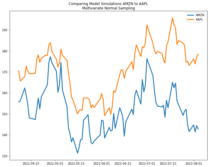
As we can see here, these two sample paths move almost perfectly together. Now let's use our stock model for each stock and see what two sample paths looks like:

Something isn’t quite right with our model as the correlation of the real stocks is not reflected here.

As we can see in this example, these two simulated versions of AMZN and AAPL don't at all seem to be a closely connected in behavior. This is of course, because the model has no information about this correlation between these two prices.

Multivariate Normal as a stock model

The solution to our problem is just a minor step up in sophistication: instead of modeling our individual stock prices as separate normal distributions, we model all of them as a single multivariate normal. The difference of course is that rather than a standard normal modeled as a mean \(\mu\) and standard deviation \(\sigma\), the multivariate normal is parametrized with a vector of means \(\mathbf{\mu}\) and a covariance matrix \(\mathbf{\Sigma}\). We can estimate these parameters using the following basic tools in numpy:

mu_amzn_aapl = ret_data[['AMZN','AAPL']].mean()
cov_amzn_aapl = ret_data[['AMZN','AAPL']].cov()

As we can see the covariance matrix captures not only the way the individual log stock returns vary over time, but also how they vary with each other.

> cov_amzn_aapl
          AMZN      AAPL
AMZN  0.001383  0.000712
AAPL  0.000712  0.000595

Now when we plot out two random samples we can see the price movements are correlated in a very similar way to the original data!

Modeling with a multivariate normal does a much better job of capturing the correlation in price movements.

While moving from two univariate normals to a single multivariate normal is a fairly simple change, we will soon see this becomes an essential aspect of optimally stock portfolios.

Modern Portfolio Theory

On the surface MPT just amounts to optimization of weights for stocks represented in by a multivariate normal. However, looking at purely the math and the optimization (which we shall do shortly), it is easy to miss the magic of what's really happening behind this somewhat simple mathematical model.

Comparing Correlated, Uncorrelated and Negatively Correlated Assets

For this section we'll start comparing alternate cases for our AAPL and AMZN portfolio. We'll assume that each stock is weighted the same, and we'll be focused on the average log returns for the day.

Note: the E[log(x)] is not the same as the log(E[X]), however we will be staying in log returns for the rest of this post and the ultimate difference is not too big. Most importantly all the relationships we find will hold in either case.

We can start by visualizing the cumulative sum of the average daily log returns for our observed data:

Had we had this portfolio this is what our cumulative log returns would have look like.

Next we can consider two alternate cases of our model. One where AMZN and AAPL are not correlated, and one where they are negatively correlated. Here is the code to create these alternate scenarios. We'll also change our expectations to be positive here, just so in this example we can actually hope to make some money!

# negatively correlated
cov_amzn_aapl_neg = np.array([[1,-1],
                              [-1,1]])*cov_amzn_aapl
# uncorrelated
cov_amzn_aapl_uncor = np.array([[1,0],
                                [0,1]])*cov_amzn_aapl

# postive returns (because that's more fun)
mu_amzn_aapl_pos = np.abs(mu_amzn_aapl)

Now we can model 3 different scenarios. We'll sample 1000 times from each of these models for the correlated, uncorrelated and negatively correlated portfolios. Then we’ll also look at the total returns at the end of each sample path and compare these distributions for all three cases:

While the expectations of all of these are the same, there is a major difference in variance of the final outcome

As we can see visually here, while all of these sample portfolios have the same expected return, there is wildly different variance depending on whether or not our assets are have correlated, uncorrelated or negatively correlated returns. Given equal expectation, we would much prefer uncorrelated returns.

Modeling this problem mathematically

We can save a lot of time spent running simulations if we look at our portfolio a bit more mathematically.

What we know

We'll start by assuming a vector of weights (summing to 1) representing the percentage of each asset that makes up our total portfolio. We'll note this with \(\mathbf{w}\).

Then we have a vector of the expected return \(\mathbf{r}\) of each asset in the portfolio. This is the sample as our mu_amzn_aapl, that is the means of the multivariate normal representing all possible assets.

And of course we also have our covariance matrix \(\mathbf{\Sigma}\).

Finally we might want to consider the number of days we are modeling \(N\).

What we calculate

Now we can take these basic pieces and put together the foundations of the method we'll be using to find an optimal portfolio.

The heart of what we what to know is what our expected return will be after \(N\) days, given the rest of our information, we'll call this \(\mu_{p}\):

$$\mu_{p} = \mathbf{w}^T \mathbf{r} \cdot N$$

Next we want to compute the variance in these returns, which we'll call \(\sigma_{p}^2\):

$$\sigma_{p}^2 = \mathbf{w}^T(\Sigma \cdot N) \mathbf{w}$$

and of course our volatility or standard deviation \(\sigma_p\) is just:

$$\sigma_p = \sqrt{\sigma_{p}^2}$$

Finally we have the Sharpe ratio which we'll use to summarize this balance between returns and volatility:

$$\text{SR}=\frac{\mu_p}{\sigma_p}$$

We can go ahead and put all of this into code. Note we'll be using JAX here rather than standard numpy because we're going to be making use of differentiable programming to optimize our original portfolio later on. Also note that we're using a softmax when we apply the weights to ensure they always sum to one.

N = stock_data.shape[0]

def exp_r_and_cov(ret_m):
    r = jnp.mean(ret_m, axis=1)
    cov_m = cov_m = jnp.cov(ret_m)
    return r, cov_m

def ret_and_vol(w, r, cov_m):
    #ensure our weights sum to 1
    w = jax.nn.softmax(w)
    ex_ret = jnp.dot(w.T,r) * N
    ex_vol = jnp.sqrt(jnp.dot(w.T, jnp.dot(cov_m * N,w)))
    return (ex_ret,ex_vol)

def sharpe(ex_ret, ex_vol):
    sr = ex_ret/ex_vol
    return sr

Now, rather than run simulations, we can quickly compare the information we have about what we expect our final return distribution to look like:

Corr ret: 0.07028846442699432, vol: 0.2640809714794159, SR: 0.26616254448890686
Uncorr ret: 0.07028846442699432, vol: 0.20138496160507202, SR: 0.3490253984928131
Neg corr ret: 0.07028846442699432, vol: 0.10664453357458115, SR: 0.6590911149978638

As we can see, our negatively correlated assets have the highest Sharpe ratio.

Finally we can put all of this together and create an optimal portfolio of all 12 stocks we're looking at.

Optimizing our portfolio

It should be clear now that the only thing left for us to do is figure out the best combination of weights that provide the highest Sharpe ratio for our entire portfolio.

We'll start by sampling some weights and looking at what we get from multiple resamples. here is what the code will look like for sampling:

rng = np.random.default_rng(1337)
X = jnp.array(ret_data.T)
w = rng.random(ret_data.shape[1])
w = jax.nn.softmax(w)

And here we can see the results of a random search of our weight space:

We should be able to do much better than just throwing darts at a board. Let's use JAX and find our optimal portfolio!

Optimization with differentiable programming

Because we wrote all of our code using JAX it's very straight forward to create our loss function:

def sharpe_loss(w, ret_m):
    r, cov_m = exp_r_and_cov(ret_m)
    ex_ret, ex_vol = ret_and_vol(w, r, cov_m)
    sr = sharpe(ex_ret, ex_vol)
    return -sr

With this function written, we can just use JAX's grad and jit to get a compiled version of our gradient function.

d_sharpe_loss_wrt_w = jit(grad(sharpe_loss,argnums=0))

Do demonstrate our progress, we can show the initial distribution of asset weights in a randomly selected portfolio:

Our initial weights give us a Sharpe ratio of 0.173

Notice that the Sharpe ratio of this portfolio is 0.173.

To find a better portfolio we just use a very simple gradient descent algorithm to improve our guess.

lr = 1.0
for step in range(500):
  w_grad = d_sharpe_loss_wrt_w(w,X)
  w -= lr*w_grad
  if step % 100 == 0:
    print(f"grad l2 ")
    print(f"step  - Sharpe:{-sharpe_loss(w, X)}")

Finally we can take a look at our optimized portfolio!

Now we see a much better Sharpe ratio and very different portfolio.

With a Sharpe ratio of 1.38 we've made significant improvement over our initial portfolio!

Conclusion

Before going further I want to give a shout out to Yves Hilpisch's Python for Finance, which was the book that really made MPT click for me.

What I find remarkable about MPT is both its simplicity and hidden depth. On the surface it's a remarkably simple weighting of a multivariate normal. If you look at just the mathematics, it's not immediately obvious that this algorithm is essentially poring over all the many possible ways that different assets correlate with one another and optimizing for how this impacts the variance of their expected returns.

All that said, it's important to remember that the biggest assumption of this model is that future returns can be predicted by past performance. For all the cleverness and beauty of quantitative finance, this is a persistent issue in many of the models.

Nonetheless I find Modern Portfolio Theory incredibly fascinating and another fun example of where we can use JAX and differentiable programming to help solve an optimization problem by essentially just describing our problem in code.

Support on Patreon

Support my writing on Patreon and gain access to the source code and video commentary for this article as well as access to much more of my writing!