In this post we're going to take a look at a way of comparing two probability distributions called Kullback-Leibler Divergence (often shortened to just KL divergence). Very often in Probability and Statistics we'll replace observed data or a complex distributions with a simpler, approximating distribution. KL Divergence helps us to measure just how much information we lose when we choose an approximation.

Let's start our exploration by looking at a problem. Suppose that we're space-scientists visiting a distant, new planet and we've discovered a species of biting worms that we'd like to study. We've found that these worms have 10 teeth, but because of all the chomping away, many of them end up missing teeth. After collecting many samples we have come to this empirical probability distribution of the number of teeth in each worm:

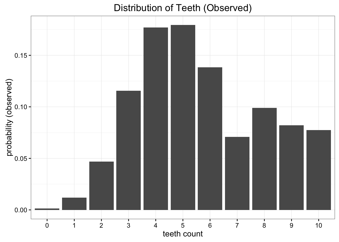
The empirical probability distribution of the data collected

While this data is great, we have a bit of a problem. We're far from Earth and sending data back home is expensive. What we want to do is reduce this data to a simple model with just one or two parameters. One option is to represent the distribution of teeth in worms as just a uniform distribution. We know there are 11 possible values and we can just assign the uniform probability of $\frac{1}{11}$ to each of these possibilities.

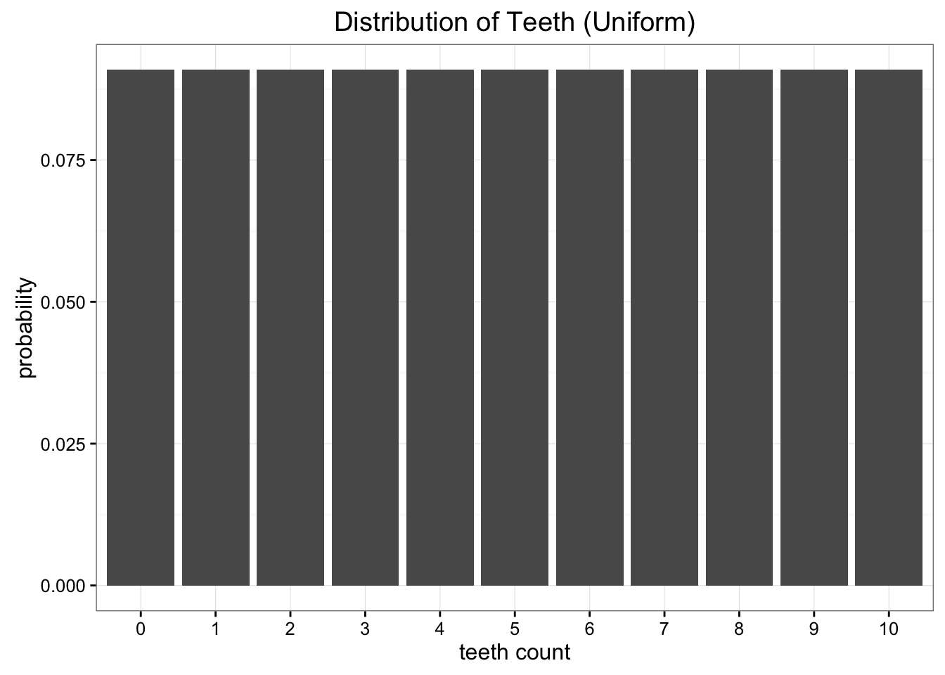
Our uniform approximation wipes out any nuance in our data

Clearly our data is not uniformly distributed, but it also doesn't look too much like any common distributions we know. Another option we could try would be to model our data using the Binomial distribution. In this case all we need to do is estimate that probability parameter of the Binomial distribution. We know that if we have $n$ trials and a probabily is $p$ then the expectation is just $E[x] = n \cdot p$. In this case $n = 10$, and the expectation is just the mean of our data, which we'll say is 5.7, so our best estimate of p is 0.57. That would give us a binomal distribution that looks like this:

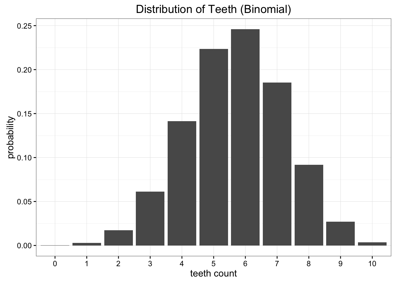
Our binomial approximation has more subtlety, but doesn't perfectly model our data either

Comparing each of our models with our original data we can see that neither one is the perfect match, but which one is better?

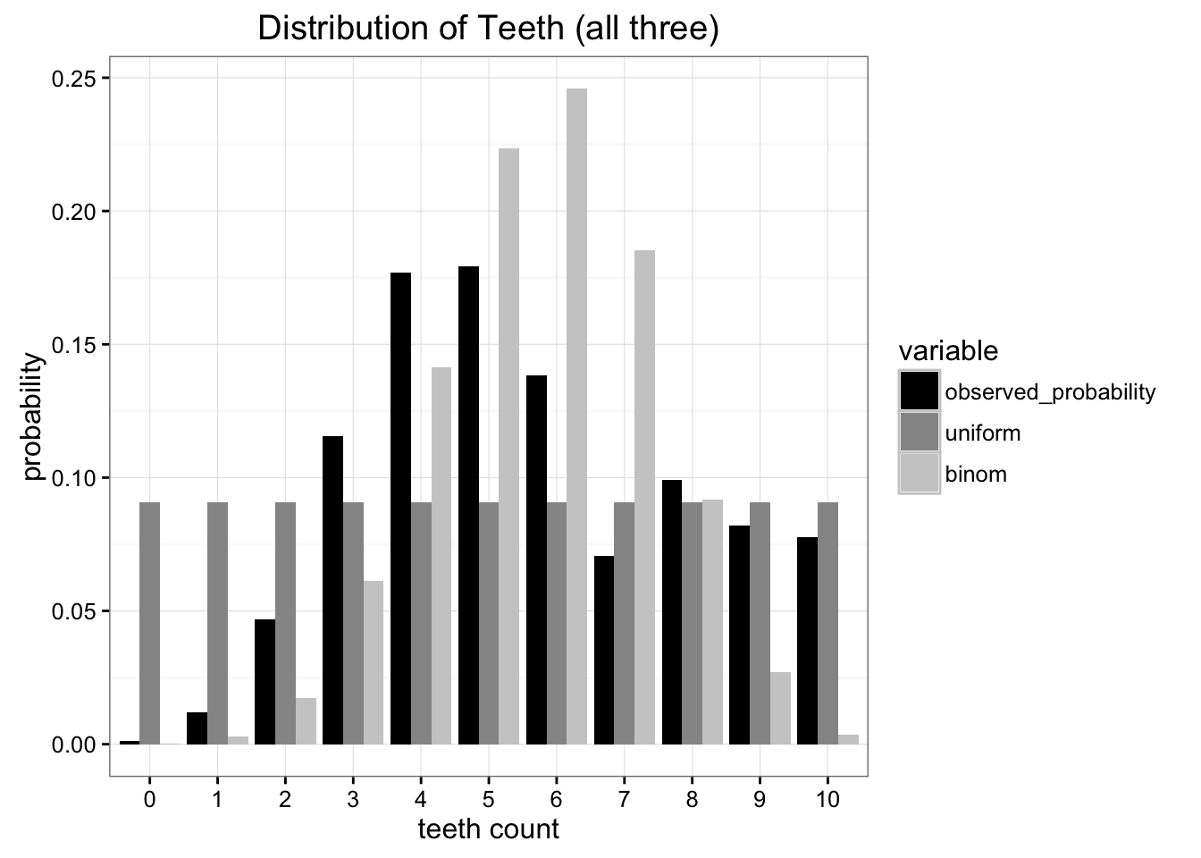
Compared with the original data, it's clear that both approximations are limited. How can we choose which one to use?

There are plenty of existing error metrics, but our primary concern is with minimizing the amount of information we have to send. Both of these models reduce our problem to two parameters, number teeth and a probability (though we really only need the number of teeth for the uniform distribution). The best test of which is better is to ask which distribution preserves the most information from our original data source. This is where Kullback-Leibler Divergence comes in.

The entropy of our distribution

KL Divergence has its origins in information theory. The primary goal of information theory is to quantify how much information is in data. The most important metric in information theory is called Entropy, typically denoted as $H$. The definition of Entropy for a probability distribution is:

$$H = -\sum_{i=1}^{N} p(x_i) \cdot \text{log }p(x_i)$$

If we use $log_2$ for our calculation we can interpret entropy as "the minimum number of bits it would take us to encode our information". In this case, the information would be each observation of teeth counts given our empirical distribution. Given the data that we have observed, our probability distribution has an entropy of 3.12 bits. The number of bits tells us the lower bound for how many bits we would need, on average, to encode the number of teeth we would observe in a single case.

What entropy doesn't tell us is the optimal encoding scheme to help us achieve this compression. Optimal encoding of information is a very interesting topic, but not necessary for understanding KL divergence. The key thing with Entropy is that, simply knowing the theoretical lower bound on the number of bits we need, we have a way to quantify exactly how much information is in our data. Now that we can quantify this, we want to quantify how much information is lost when we substitute our observed distribution for a parameterized approximation.

Measuring information lost using Kullback-Leibler Divergence

Kullback-Leibler Divergence is just a slight modification of our formula for entropy. Rather than just having our probability distribution $p$ we add in our approximating distribution $q$. Then we look at the difference of the log values for each:

$$D_{KL}(p||q) = \sum_{i=1}^{N} p(x_i)\cdot (\text{log }p(x_i) - \text{log }q(x_i))$$

Essentially, what we're looking at with the KL divergence is the expectation of the log difference between the probability of data in the original distribution with the approximating distribution. Again, if we think in terms of $log_2$ we can interpret this as "how many bits of information we expect to lose". We could rewrite our formula in terms of expectation:

$$D_{KL}(p||q) = E[\text{log } p(x) - \text{log } q(x)]$$

The more common way to see KL divergence written is as follows:

$$D_{KL}(p||q) = \sum_{i=1}^{N} p(x_i)\cdot log\frac{p(x_i)}{q(x_i)}$$

since $\text{log }a - \text{log b} = \text{log }\frac{a}{b}$.

With KL divergence we can calculate exactly how much information is lost when we approximate one distribution with another. Let's go back to our data and see what the results look like.

Comparing our approximating distributions

Now we can go ahead and calculate the KL divergence for our two approximating distributions. For the uniform distribution we find:

$$D_{kl}(\text{Observed } || \text{ Uniform}) = 0.338$$

And for our Binomial approximation:

$$D_{kl}(\text{Observed } || \text{ Binomial}) = 0.477$$

As we can see the information lost by using the Binomial approximation is greater than using the uniform approximation. If we have to choose one to represent our observations, we're better off sticking with the Uniform approximation.

Divergence not distance

It may be tempting to think of KL Divergence as a distance metric, however we cannot use KL Divergence to measure the distance between two distributions. The reason for this is that KL Divergence is not symmetric. For example we if used our observed data as way of approximating the Binomial distribution we get a very different result:

$$D_{kl}( \text{Binomial} || \text{Observed}) = 0.330$$
Intuitively this makes sense as in each of these cases we're doing a very different form of approximation.

Optimizing using KL Divergence

When we chose our value for the Binomial distribution we chose our parameter for the probability by using the expected value that matched our data. But since we're optimizing for minimizing information loss, it's possible this wasn't really the best way choose the parameter. We can double check our work by looking at the way KL Divergence changes as we change our values for this parameter. Here's a chart of how those values change together:

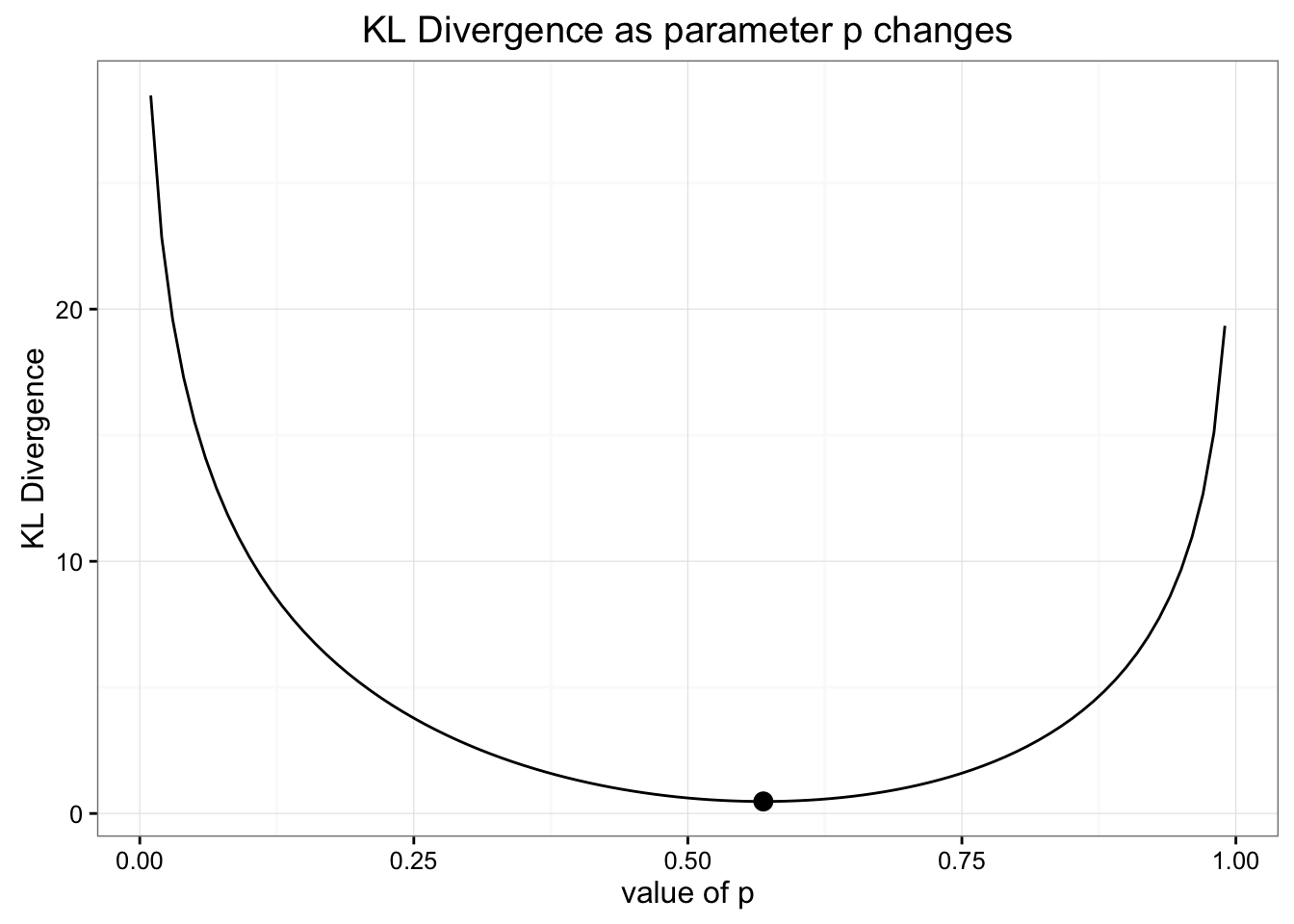
It turns out we did choose the correct approach for finding the best Binomial distribution to model our data

As you can see, our estimate for the binomial distribution (marked by the dot) was the best estimate to minimize KL divergence.

Suppose we wanted to create an ad hoc distribution to model our data. We'll split the data in two parts. The probabilities for 0-5 teeth and the probabilities for 6-10 teeth. Then we'll use a single parameter to specify what percentage of the total probability distribution falls on the right side of the distribution. For example if we choose 1 for our parameter then 6-10 will each have a probability of 0.2 and everything in the 0-5 group would have a probability of 0. So basically:

$$[6,11] = \frac{p}{5}; [0,5] = \frac{1-p}{6}$$

Note: Because $log$ is undefined for 0, the only time we can allow probabilities that are zero is when $p(x_i) = 0$ implies $q(x_i) = 0$.

How could we find the optimal parameter for this strange model we put together? All we need to do is minimize KL divergence the same way we did before:

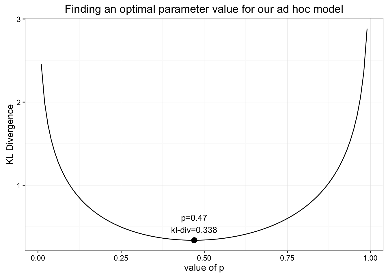
By finding the minimum for KL Divergence as we change our parameter we can find the optimal value for p.

We find that the minimum value for KL Divergence is 0.338 found when $p=0.47$. That value for the minimum KL divergence should look pretty familiar: it's nearly identical to the value we got from our uniform distribution! When we plot out the values of our ad hoc distribution with the ideal value for $p$ we find that it is nearly uniform:

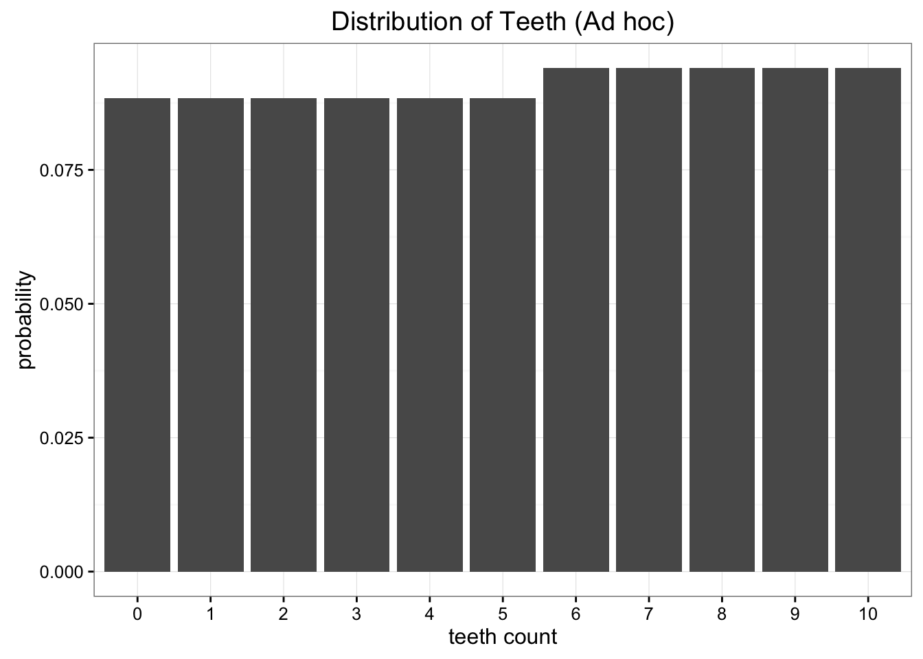
Our ad hoc model ends up being optimal very close to the uniform distribution

Since we don't save any information using our ad hoc distribution we'd be better off using a more familiar and simpler model.

The key point here is that we can use KL Divergence as an objective function to find the optimal value for any approximating distribution we can come up with. While this is example is only optimizing a single parameter, we can easily imagine extending this approach to high dimensional models with many parameters.

Variational Autoencoders and Variational Bayesian methods

If you are familiar with neural networks, you may have guessed where we were headed after the last section. Neural networks, in the most general sense, are function approximators. This means that you can use a neural network to learn a wide range of complex functions. The key to getting neural networks to learn is to use an objective function that can inform the network how well it's doing. You train neural networks by minimizing the loss of the objective function.

As we've seen, we can use KL divergence to minimize how much information loss we have when approximating a distribution. Combining KL divergence with neural networks allows us to learn very complex approximating distribution for our data. A common approach to this is called a "Variational Autoencoder" which learns the best way to approximate the information in a data set. Here is a great tutorial that dives into the details of building variational autoencoders.

Even more general is the area of Variational Bayesian Methods. In other posts we've seen how powerful Monte Carlo simulations can be to solve a range of probability problems. While Monte Carlo simulations can help solve many intractable integrals needed for Bayesian inference, even these methods can be very computationally expensive. Variational Bayesian method, including Variational Autoencoders, use KL divergence to generate optimal approximating distributions, allowing for much more efficient inference for very difficult integrals. To learn more about Variational Inference check out the Edward library for python.

Bayesian Statistics the Fun Way is out now!

If you want to learn more about Bayesian Statistics and probability: Order your copy of Bayesian Statistics the Fun Way No Starch Press!

If you enjoyed this writing and also like programming languages, you might enjoy my book Get Programming With Haskell from Manning.