Prior Probability in Logistic Regression
In the last post we looked at how we can derive logistic regression starting from Bayes' Theorem. In this post we're going to explore this a bit further by looking at how prior probabilities are learned by our logistic model. The prior probability for our \(H\) is directly related to the class balance in our training set. This is important because it can lead to logistic regression models behaving in unexpected ways if we are trying to predict on data with a different class imbalance than we trained on. Luckily, because at its heart logistic regression in a linear model based on Bayes’ Theorem, it is very easy to update our prior probabilities after we have trained the model.
As a quick refresher, recall that if we want to predict whether an observation of data D belongs to a class, H, we can transform Bayes' Theorem into the log odds of an example belonging to a class. Then our model assumes a linear relationship between the data and our log odds:
$$lo(H|D) = \beta D + \beta_0$$
Which, when transformed back into a probability gives us the familiar form of logistic regression:
$$P(H|D) = \frac{1}{1+e^{-(\beta D + \beta_0)}}$$
If this refresher is not clear, definitely go back and read through the first post.
Prior probabilities and logistic regression
To demonstrate how useful understanding the relationship between Bayes' Theorem and logistic regression is, we'll look at a practical problem that this insight helps us solve. The previous post on this topic had us using logistic regression to predict whether the setup for brewing a cup of coffee would lead us to a good cup. Suppose when I started training my coffee model I was pretty awful at coming up with brewing setups and only 1 in 10 of my cups of coffee was really great. This means that in the training data we had an imbalance in the number of positive to negative examples. What impact is this going to have on our model?
Imagine this setup. I have 100 training examples of my data \(D\), 10 observations of 1 (good cups of coffee) and 90 observations of 0 (bad cups of coffee). This is going to impact what the model learns in a very predictable way. If you go back to our odds version of logistic regression we were trying to learn:
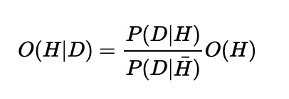
The \(O(H)\), is our prior odds, which means "given we know nothing else about the problem, what are the odds of H". Intuitively if we train the model on 10 examples of \(H\) and 90 examples of \(\bar\), then we expect:
$$O(H) = \frac{10}{90}$$
And of course we can convert this into a probability using the rule mentioned earlier:
$$P(H) = \frac{O(H)}{1+O(H)} = 0.1$$
This result isn't surprising since we know 10 out of 100 cases was positive, so 0.1 seems like the best estimate for our prior probability.
This also means that \(\beta_0\) in our log odds model then corresponds to the log odds of the prior since it takes the place of \(O(H)\) when we finally log transform our problem. The result of this is that whenever you train a logistic model, if you have \(N_1\) observations of class 1 and \(N_0\) observations of class 0, then \(\beta_0\) should be approximately:
$$\beta_0 = log \frac{N_1}{N_0}$$
Or another way to say this is that:
$$P(H) = \frac{N_1}{N_1+N_0}$$
So...
$$\beta_0 = log \frac{P(H)}{1-P(H)}$$
However we look at it, the best estimate for the prior probability of H is just to look at the ratio of positive observations in our training data, and since \(\beta_0\) is literally the log odds of our prior, we know that this estimate will the log odds of the ratio of positive examples in the training data.
A proof and some practical details
In practice (and theory!) you'll need to center your training data for this relationship between \(\beta_0\) and log odds prior to hold. Centering means that the mean of of each column of \(D\) is 0 (this is achieved simply by subtracting the mean of each column from each value column in your training data). As a quick, intuitive proof we can look at what happens when we compute the expectation of our log odds model. If we have centered our data the expectation is what we would expect to happen on average given we know nothing else about our problem. This is also a great definition for the concept of prior probability: what we expect to happen given we know nothing else about our problem. In the case of making cups of coffee, if we know that only 1 in 10 are good, and we know nothing else about our brewing set up, we would expect the probability of a good cup is 0.1.
We can see that this is also mathematically the case when we compute the expectation for our centered data. Expectation for our logistic model is:
$$E[lo(H|D)] = E[\beta D+\beta_0]$$
We can expand the right side of this equation in the following way.
$$E[\beta D+\beta_0] = E[\beta D] + E[\beta_0]$$
$$E[\beta D] + E[\beta_0] = \beta E[D] + E[\beta_0]$$
And recall that \(\beta_0\) is a constant so \(E[\beta_0] = \beta_0\)
Now since we centered our data, by definition \(E[D] = 0\), which leaves us with:
$$E[lo(H|D)] = \beta E[D] + \beta_0 = \beta \cdot 0 + \beta_0 = \beta_0$$
So, if we centered our data, the expectation for our model, which is the same thing as what we mean by "the prior probability" for our model, is just the constant \(\beta_0\). And, given our training data, we know that the best estimate for \(\beta_0\) is the log ratio of positive to negative training examples.
Changing the prior after training the model!?
We now know how prior information about a class will be incorporated into our logistic model. Assume that I've been using this model trained on 100 examples with 10 positive and 90 negative examples. However, with time, my knack for making coffee really improves and now I feel that my prior probability for making a great cup of coffee is 0.5, not 0.1.
I want to try a new brewing setup and I put my configuration into my model and I get this:
$$P(H|D) = 0.3$$
I trust my model, but I know that my model has also incorporated an older prior which I personally no longer believe in. This means that my model must be underestimating the probability that this will be a great cup of coffee. And unfortunately, I've decided to host my model in some cloud service so I no longer have access to any of it's parameters, I can only give it input and receive its output.
I no longer trust the output of this model because my prior beliefs have changed. Since logistic regression is just an application of Bayes' Theorem, shouldn't I be able to update my prior probability?
We have in our hand \(P(H|D)\) which is 0.3, and all we want to change is our prior, which we know is \(\beta_0\). Recall that according to our logistic model, \(P(H|D)\) is defined as follows:
$$P(H|D) = \frac{1}{1+e^{-(\beta D + \beta_0)}}$$
All we need to do is to somehow replace \(\beta_0\) with the updated prior log odds, which we'll call \(\beta'_0\). If we had access to our coefficients \(\beta \) then we could simply recompute everything, but we only have the model's prediction of 0.3. It turns out there is an easier way to solve this than recomputing our model's prediction, that doesn't require us to know \(\beta\), we just need to know \(beta_0\) the original log odds prior (or we can estimate it as the log odds ratio of training examples). Let's look at the log odds form of our model, which we can use when our probabilities are not at the extremes of 0 or 1.
$$lo(H|D) = \beta D + \beta_0$$
We don't care about \(\beta D\), all we want to do is change \(\beta_0\) to \(\beta'_0\), and since this is just a linear equation, this is very easy:
$$\beta D + \beta'_0 = \beta D + \beta_0 + (\beta'_0 - \beta_0) = lo(H|D) + (\beta'_0 - \beta_0) $$
So if we add the \(\beta'_0 - \beta_0\) to our log odds of our class then we get an updated posterior log odds reflecting our new prior!
Let's update that prior!
First let's figure out what our value for \(\beta'_0\), should be. We just need to translate our new prior into log odds (and we'll be using natural log since our model is using \(e\)):
$$\beta'_0 = ln \frac{0.5}{1-0.05}= ln\text{ 1} = 0$$
Ah! Our new prior in log odds form is just 0, this makes our math very easy. We know the previous value for \(\beta\) should be roughly equivalent to the log of the class ratio in the training data:
$$\beta = log(\frac{10}{90}) = -2.2$$
So now we just have to subtract -2.2 from our the log odds result from our model, which is the same as adding 2.2. Right now we only have the output of our model as \(P(H|D) = 0.3\) and we need the log odds. But this is pretty easy to compute as well.
$$log(\frac{0.3}{1-0.3}) = -0.85$$
Now we just add 2.2 to this and see that
$$\beta D + \beta'_0 = -0.85 + 2.2 = 1.35$$
So the log odds that we'll make a good cup of coffee is 1.35! We want our answer in the form of a probability. We've gone back and forth between log odds, odds and probabilities so this should be getting a bit familiar. Our new P(H|D) is:
$$P(H|D) = \frac{e^{1.35}}{1+e^{1.35}} = 0.79$$
When we update our prior we get a new prediction that says we're much more likely to get a great cup of coffee out of our brew! The amazing thing here is that we were able to update our prior after the model made a prediction simply by knowing what our original prior was and understanding how the logistic model works!
Next we'll look at another example were we can change an entire group of predictions from a model. We'll also see how the distribution of predictions changes when we do prior updating in bulk.
Bayes' Pox and Frequentist Fever!
We saw how to fix the case of an individual estimate from a model, but now let's look at what happens to a larger collection of estimates when a model is trained with one prior and predicted on a population with a different prior. In this example we'll use real (simulated) data and train an actual logistic model in R to see how all of this works.
Everyone gets sick of statistics sometimes and this can result in two major illnesses: Frequentist Fever or Bayes' Pox. Each disease shares common symptoms but with different rates.

Fever
Runny Nose
Cough
Headache
Bayes bumps (easily mistaken for a pimple)
We're going to be generating data with the rates shown in the table for each of the symptoms, but we only know these true rates because we are in control of the simulated data.
Using these rates for symptoms we are going to generate a train data set and a test data set. Now we’re going to assume that our training data, train.data comes from the Institute of Statistical Illnesses and has 1000 examples. However, the Institute of Statistical Illnesses tends to be a bit over eager in their recordings of Bayes' Pox so 90% of the sample data is cases of Bayes' Pox.
We want to build a model that learns to predict Bayes' Pox given the data we have. Here is the R code for a logistic model using the glm function. We've also already gone ahead and centered our training data (and recorded the column means so we can center our test data in the same way):
bayes.logistic <- glm(bayes_pox ~ 1 + fever + runny_nose +
                      cough + headache + bayes_bumps,
                      data=train.data,family=binomial())
Now that we've trained our model we can inspect it to see that it has learned what we would expect it to have learned regrading the prior.
model.summary <- summary(bayes.logistic)
The first coefficient tells us what our model's estimate for the intercept, \(\beta_0\) is. We can see that model.summary$coefficients[1][1] = 1.8. Remember that this value represents the log odds of our prior. If we want to convert this back to a probability we just need to use the logistic function. We can see that logistic(model.summary$coefficients[1][1]) = 0.86 which is pretty close to our 90% prior probability of Bayes' Pox that is represented in the data.
Assumptions about Beta_0 and Priors
Why isn't it exactly 0.9? This is for a couple of reasons. Our model is not a perfect representation of our problem. Remember that we must center our data in order for \(\beta_0\) to truly represent our prior. This is because we want the expectation of our data to be 0. If all of our data was normally distributed continuous values then we should see \(\beta_0\) be very close to the true prior. However, when we represent our symptoms they only take on values of 1 or 0. When we center our data we subtract the means for these but we still only have two values. This leads to the model not quite making perfect estimates as far as prior probabilities go. We also have to think of what it means for all of our data to be 0, even when scaled. Does this really represented the “average” case? What is an “average” symptom?
Nonetheless, our model learned prior, \(\beta_0\), is pretty close to what we would expect it to be. This means we can go ahead and update it with a new prior if we need to.
But Bayes' Pox is rare!
So far we have used the training data to come up with a model to detect whether or not a sick statistician has Bayes' Pox or Frequentist Fever. But there's a problem. Unsurprisingly, people get sick far less frequently from Bayesian statistics than Frequentist statistics and so Bayes' Pox is actually much less common. Only 0.01 of the sick statisticians have Bayes' pox, but our model has learned a prior probability that Bayes' Pox is more likely. Let's see how our model predicts on a set of test.data that has only about 1% of the population having Bayes' pox.
We can use R to make new predictions on the 100,000 test cases of sick statisticians:
model.preds <- predict(bayes.logistic,test.data,type="response")
If we plot these predictions out we can see the distribution of what we think is happening:

The distribution of the prediction for our logistic model given the prior in the training data.
It does look like most statisticians are still being diagnosed as not having Bayes' Pox, but how does our model predict when trained on the wrong prior? Here is a plot showing what the observed rate of Bayes Pox are when we look at different thresholds for determining "has Bayes' Pox". In the ideal case this would be a straight line with a slope of 1, indicating that our model's certainty corresponds with the empirical ratio of Bayes' Pox and Frequentist Fever. That is, if the model is making a prediction of 0.5 we would hope that roughly half the time it's right, if the model predicts 0.99 we would hope that 99% of those predictions are, in fact, Bayes' Pox.

Because it is trained on the wrong prior, the model drastically overestimates the empirical rate of Bayes’ Pox.
We know our model isn't perfect and we also know that you can't always be right in probability. However, what we can see clearly here is that our model, with the original prior, wildly overestimates the chance of having Bayes' Pox. Take for example the 0.5 model probability. This is the point where the model is telling us that it is equally likely that the observation is Bayes' Pox as it is Frequentist Fever. We can clearly see that in the cases where the model is uncertain, Bayes' Pox is far less likely than Frequentist Fever. In many software packages 0.5 is the default threshold for deciding on a class, and in this case we would be wildly over predicting Bayes' Pox.
Adjusting our prior
The problem here is that our model assumes that the prior probability of having Bayes' Pox is very high based on an inaccurate distribution of Bayes' Pox cases in our train.data. We can correct this the same way we solved our coffee model problem. This time, rather than walk through the process of transforming probability to odds and odds to log odds (and back), we'll use the logit function to transform probabilities to log odds and logistic to turn them back (we're using these functions as defined in the rethinking package).
Let's start fixing our problem by transforming our model.preds back into the log odds form:
lo.preds <- logit(model.preds)
From our earlier notation, lo.preds are the \(lo(H|D)\) or \(\beta D + \beta_0\).
If we have access to the actual model and it's parameters we can get \(\beta_0\) directly:
model.prior.lo <- model.summary$coefficients[1][1]
The next step is that we need to calculate what the correct log odds should be. If we know that the probability of having Bayes' Pox among sick statisticians is only 0.01 we can represent this as, our \(\beta_0'\) from earlier:
correct.lo <- logit(0.01)
With this information we can update our log odds predictions as we did before, \(lo(H|D) + (\beta'_0 - \beta_0)\)
updated.lo.preds <- lo.preds + (correct.lo - model.prior.lo)
All that's left now is to convert this log odds updated predictions back to probabilities using logistic:
updated.preds <- logistic(updated.lo.preds)
The update.preds represents our model with the correct prior probability used to calculate whether or not a sick statistician has Bayes' Pox. Plotting this out we can see that the impact on the distribution of predictions is striking:

Distribution of predictions after updating our prior to the correct one.
Our change didn't just shift our predictions over, it completely changed the shape of the distribution! This is because we did our transformation in log space and then transformed the data back. So using the wrong prior doesn't simply make our predictions off by a constant factor but really changes the shape of our distribution.
Improved predictions
We can now revisit the empirical ratio of Bayes' Pox to Frequentist Fever with our new thresholds:

With our updated prior, our model’s beliefs are much closer to the empirical ratio of Bayes’ Box to Frequentist Fever.
Here we see that our model's adjusted predictions are much closer to its actual rate of being correct. Our model, of course, isn't perfect, but we'll be scaring far less people with a false diagnosis of Bayes' Pox.
Even though the shape of our distribution changed quite a bit with our updated prior, the ordering of our predictions did not. In practice we would likely want to choose a threshold for our model that optimized trade offs between precision and recall (our plot here only shows the precision). Still this serves as a practical example of how a prior learned in training can impact the way our model interprets the world. Using the correct prior is especially important if we want to interpret the output of a logistic model as an actual degree of belief in our hypothesis (as opposed to just an arbitrary prediction threshold).
Conclusion
In industry it is very often the case that logistic models are a great solution for a classification problem, and almost always a good place to start. It is common practice to train logistic models on balanced training sets even when it is known that one class is far less likely to occur than the other. What many people using logistic models fail to recognize is that the training data will have an impact on what your model learns is the prior probability of each class. Luckily it is very easy to transform prediction from a model to use a different prior than the model was trained with. This adjustment will aid in the interpretability of model predictions.
A special thanks for this post goes out the a former coworker of mine John Walk who got me thinking about this problem with a very interesting interview question!

Bayesian Statistics the Fun Way is out now!
If you enjoyed this post please subscribe to keep up to date and follow @willkurt!
If you want to learn more about Bayesian Statistics and probability: Order your copy of Bayesian Statistics the Fun Way No Starch Press!
If you enjoyed this writing and also like programming languages, you might enjoy my book Get Programming With Haskell from Manning.