Why Bayesian Stats Needs Monte-Carlo Methods
This post emerged from a series of question surrounding a Twitter comment that brought up some very interesting points about how Bayesian Hypothesis testing works and the inability of analytic solutions to solve even some seemingly trivial problems in Bayesian statistics.
Comparing Beta distributed random variables is something that comes up pretty frequently on this blog (and in my book as well). The set up is fairly straight forward: model an A/B test as sampling from two beta distributions, sample from each distribution a lot, then compare the results.
This simulation approach often first appears as a clever little trick to solve a more complex math problem, but in fact is a primative form of Monte-Carlo Integration and turns out to one of the only ways to really solve this problem. By exploring this topic deeper in this post we'll see some of the myths that many people have about analytic solutions as well as demonstrating why Monte-carlo methods are so essential to Bayesian statistics.
Background: A conversation about election results
An interesting conversation happened on Twitter recently. It started with a retweet of mine regarding Nate Silver (well know author and election forecaster) posting his latest predictions for the 2020 presidential election showing that Biden has a 71% probability of winning versus Trump's 29%
After the last election there was quite a lot of criticism about Nate Silver's forecasting since his company (538) predicted that Hilary Clinton would win with a probability of 71% in the 2016 presidential election.
This criticism has always annoyed me personally since, in statistical terms, 71% is generally not considered a strong belief in anything. So it is not inconsistent, nor suprising for someone to believe a candidate has 71% chance of success and they still lose. Even when looking at typical p-values, we wait for 95% percent certainty before making claims (and many feel this is a pretty weak belief). But for some reason whenever election polls come up, it seems even very statistically minded people suddenly think that 51% chance is a high probability.
I retweeted Nate Silver's forecast, mentioned my annoyance and provided an example of another case with a similar probability of winning:
If you were running an A/B test and your A variant had 2 success in 15 trials and your B variant had 3 successes in 14 trails, you would be roughly 71% confident that B was the superior variant.
Even someone without much statistical training would likely be very skeptical of such a claim, but somehow during election forecasts even experience statisticians can look at Silver's post and think that Biden winning is a sure thing.
How do we arrive at P(B > A)?
Twitter user @mbarras_ing ask a really important follow up question, asking to explain this result:
I very strongly believe that all statistics, even quick off the cuff estimates, should be reproducible and explainable.
I've written a fair bit about approaching similar problems both on this blog and in my book. The big picture is that we're going to come up with parameter estimates for the rate that A and B convert users and then compute the probability that B is greater than A.
Since we're estimating conversion rates we're going to use the Beta distribution as the distribution of our parameter estimate. In this example I'm also assume a \(\text{Beta}(1,1)\) prior for our A and B variants.
The likelihood for A is \(\text{Beta}(2,13)\) and for B is \(\text{Beta}(3,11)\) so we can represent A and B as two random variables samples form these posteriors:
$$A \sim \text{Beta}(2+1, 13+1)$$
$$B \sim \text{Beta}(3+1,11+1)$$
We can now represent this in R, and sample from these distributions:
N <- 10000
a_samples <- rbeta(N,2+1,13+1)
b_samples <- rbeta(N,3+1,11+1)
And finally we can look at the results of this to compute the probability that B is greater than A:
sum(b_samples > a_samples)/N
In this case we get 0.7028 pretty close to 71% for Nate Silver’s problem.
Can we solve this without R?
This explains where we get our probabilities from, but there is an obvious question that comes up when you see this result, one raised by @little_rocko
This question is interesting because it asks two questions that don't necessarily have to be related:
- is there an easy way to solve this
- is there a non-"brute force" way solve this
Before moving on I want to mention that this little snippet of R involves a lot more abstraction then it seems at first glance. What we are really doing here is equalivant to using a Monte-Carlo simulation to integrate over the distribution of the difference between two Beta distributed random variables. After the next two sections it will be more clear that what's happening here is a surprisingly sophisticated operation that is, in my opinion, the easiest method of solving this problem as well as not truly a brute force solution.
Analytic versus Easy
When we see computational solutions to mathematical problems our first instinct is typically to feel that we are avoiding solving the problem analytically. An analytical solution is one that uses mathematical analysis to find a closed form solution.
A strivial example, suppose I wanted to find the value that minimized \(f(x) = (x+3)^2\)
In R I could brute force this by looking over a range of answers like this:
f <- function(x){
  (x+3)^2
}
xs <- seq(-6,6,by=0.031)
xs[which.min(f(xs))]
As expected we get our answer of -3, but this solution takes a bit of work: we need to know how to code and we need a computer. It's also a bit messy because if we had iterated by an incredment that didn't include -3 exactly (say by 0.031) we would not get the exact answer.
If we know some basic calculus we know that our minimum has to be where the derivative is at 0. We can very easily work out that
$$f'(x) = 2(x+3)$$
And that
$$2(x + 3) = 0 $$
When
$$ x = -3 $$
Knowning basic calculus this later solution becomes much easier.
But even with the calculus is part is hard, often solving it once makes future solutions much easier. Take for example if you wanted to find the maximum likelihood for a normal distribution with a mean of \(\mu\) and standard deviation of \(\sigma\)
To solve this we start with our PDF for the normal distribution \(\varphi\):
$$\varphi(x) = \frac{1}{\sigma \sqrt{2\pi}}e^{-\frac{1}{2}(\frac{x-\mu}{\sigma})^2}$$
Now computing the derivative of this is not necessarily "easy" but it's certainly something we can do. All we really care about is when
$$\varphi'(x) = 0$$
Which we can find out happens when (computing the deriviative of course is left as an exercise for the reader):
$$\frac{\mu-x}{\sigma}$$
This allows us to reallize the amazing fact that for any normal distribution we come across, we know that the maximum likelihood estimate is the sample is when \(x = \mu\)!
Even though our calculus might take us a bit of work, once this is done the problem of doing maximum likelihood estimation for any Normal distribution truly does become easy!
Proposing an Analytic solution to our problem
Let's revisit our original problem this time attempting to find an analytic solution. This is a very interesting case because arguably this is the simplest Bayesian hypothesis test you can imagine.
Recall that we have two random variable representing our beliefs in each test. These are distributed according the the posterior which we described earlier.
$$A \sim \text{Beta}(2+1, 13+1)$$
$$B \sim \text{Beta}(3+1,11+1)$$
Here is where I skipped some steps in reasoning. What we want to know is:
$$P(B >A)$$
Which is not expressed in a particularly useful mathematical way. A better way to solve this is to consider this as the sum (or difference in this case) of two random variables. What we really want to know is:
$$P(B - A > 0)$$
In order to solve this problem we can think of a new random variable \(X\) which is going to be the difference between B and A:
$$X = B - A$$
Finally we'll suppose we have a probability density function for \(X\) we'll call \(\text{pdf}_X\). If we know \(\text{pdf}_X\) our solution is pretty close, we just need to integrate between 0 and the max domain of this distribution:
$$P(B > A) = P(B - A > 0) = \int_{x=0}^{\text{max}}\text{pdf}_{X}(x)$$
Already this is starting to look a bit complicated, but there's one big problem ahead. Unlike Normally distributed random variables, we have no equivalent of the Normal sum theorem (we'll cover this in a bit) for Beta distributed random variables.
What does \(\text{pdf}_X\) look like? For starters we know it's not a Beta distribution itself. We can see this because we know the domain (or support) of this distribution is not \([0,1]\). Because they are Beta distributed, A and B can both take on values from 0 to 1, which means the maximum result of this difference is 1 but the minimum is -1. So whatever this distribution is, its domain is \([-1,1]\) meaning it cannot be a Beta distribution.
We can use various rules about sum of random variables to determine the mean and variance of this distribution, but without knowing the exact form of this distribution we are unable to solve the integral analytically.
Here we can see that even in this profoundly simple problem the analytical solution is frustratingly evasive.
Thankfully the joy of deriving this integral can be found in this great post on Cross Validated by Corey Yanofsky. You can also find some additional exposition from Evan Miller’s post on the topic.
Brute Force vs Monte-Carlo
This brings up the next point of the question regarding a 'non-brute force' method. Coming from a computer science background, I would generally regard 'brute force' to be defined as niavely trying solutions in until you find the best. For this problem the code for that would involve interating through probabilities and then coming up with some way to analyze the results.
What we are doing in our simulation is really a form of Monte-Carlo integration. We've already established that \(P(B > A)\) is equivalent to \(\int_{x=0}^{\text{max}}\text{pdf}_{X}(x)\). Since \(\text{pdf}_{X}\) is unknown we are approximating it by sampling from the possible differences between B and A.
If may help to visualize this distribution:

If we look at the distribution of the difference of our samples we can see that it is approximating the PDF of the difference.
Now we can shade in the propotion of all the answer that in our case will be captured by sum(b_samples > a_samples)/N and we can see that we are, in fact doing integration.

Our code hides much of the complexity, but we’re really approximating this integral
So even though we have just a bit of R code, and we are doing a lot of computation, we are rather efficienty approximating the intergral \(\text{pdf}_{X}\) from 0 to 1. This is quite a bit different than a brute force method which tries candidate solutions until it finds one it is satisfied with.
It is also important to note, that this is not a clever hack but very solid numerical method of solving this problem. It may not be as accurate and efficient as solving the proper integral (thanks @FinnLindgren), but it is very easy to implement, understand and rests on a firm mathematical foundation. As we move towards increasingly sophisticated Bayesian models we continue to solve problems in a similar way but because the integration itself gets much trickier we need more sophisticated tools like Stan and PyMC3.
Normal Approximation - a consolation prize for analytical solutions.
So far we have a great defense for this sampling approach to our solution, but in practice there are still many times when we cannot afford to run even simple simulations. As an example: at one of my first data scientist jobs we wanted to implement an A/B testing tool using these Bayesian techniques, but the computations were done in JavaScript (meaning we had no rbeta function) and users did not like have any "randomness" in their results (even if it didn't impact the final conclusions).
There is a clever analytical approximation we can do when we don't want to use a simulation in this case involving two very nice properties of the normal distirbution: the ability for the Normal distribution to approximate the Beta distribution and the Normal Sum theorem.
The Normal Distribution Approximates the Beta Distribution
The Beta distribution is defined as having two parameter \(\alpha\) and \(\beta\) where \(\alpha + \beta = n\) the total number of observations. It turns out that as \(n\) grows towards inifity (and quite a bit early than that) and \(\alpha \approx \beta\) (and it doesn't need to be that close) the Beta distribution can be very nicely approximated by the Normal distribution.
Since the Normal distribution is parameterized with a mean and varaince (or standard deviation), to do this approximation we need to know two pieces of information about the Beta distribution: its expectation and its variance. With this can then determine the approximating Normal distribution very easily.
The expectedation for the Beta distribution is:
$$E[\text{Beta}(\alpha,\beta)] = \frac{\alpha}{\alpha +\beta}$$
And the variance is defined as:
$$Var[\text{Beta}(\alpha,\beta)] = \frac{\alpha \beta}{(\alpha + \beta)^2(\alpha + \beta + 1)}$$
All this means we can now approximate any Beta distribution this way:
$$\text{Beta}(\alpha,\beta) \approx \mathcal{N}(\mu=\frac{\alpha}{\alpha +\beta},\sigma=\sqrt{\frac{\alpha \beta}{(\alpha + \beta)^2(\alpha + \beta + 1)}})$$
We can see an example here by comparing Beta(50,50) to \(\mathcal{N}(0.5,0.05)\)

In many cases the Normal distribution provides a very nice approximation of the Beta distribution.
As you can see, these two distributions are virtually indistinguishable.
The Normal Sum Theorem
Recall that the problem with adding Beta distributed random variables is that we have no nice way to get the PDF of for this new random variable representing their difference. Thankfully the Normal distirbution does not have this problem. Summing up two Normally distributed random variables leaves us with a new Normally distributed random variable with easy to compute mean and standard deviation.
The Normal sum theorem tells us that:
Given two, independent, normally distributed random variables:
$$A \sim \mathcal{N}(\mu_A,\sigma_A)$$
$$B \sim \mathcal{N}(\mu_b,\sigma_B)$$
The distribution of the sum of these variables is defined as:
$$A+B = \mathcal{N}(\mu_A +\mu_B,\sqrt{\sigma_A^2 + \sigma_B^2}$$
With this we have all the tools we need to revisit our original problem using Normal approximations!
The Normal approximation of our problem
Our Posterior pdf of A is \(\text{Beta}(3, 14)\), which means we can approximate it as:
$$\mathcal{N(\mu=0.18,\sigma=0.09)}$$
We can see how well (or not) this distribution approximates our posterior:
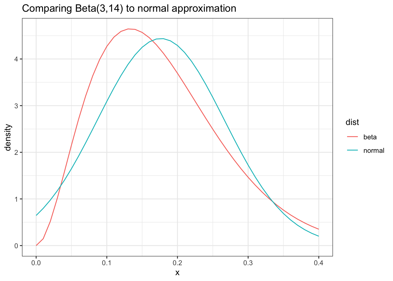
As we can see, with a low value for our total observations the Normal approximation is not that great
As we can see here this approximation is... okay. This is primarily because \(\alpha + \beta\) is still fairly small.
Nonetheless this is still the best tool we have for coming up with a nice approximation and we can ultimately compare the results of this approach with our Monte-Carlo approach.
For the posterior for B is \(\text{Beta}(4,12)\) so we will approximate it as:
$$\mathcal{N(\mu=0.33,\sigma=0.105)}$$
Finally we can come up with a Normal distirbution that represents all of the probabilities for B - A:
$$P(B-A) \approx \mathcal{N}(\mu_B -\mu_A,\sqrt{\sigma_B^2 + \sigma_A^2})$$
$$P(B-A) \approx \mathcal{N}(0.12,0.32)$$
Now let's compare this to what our sample distribution:

Our approximation for the PDF of the difference is pretty bad, but we only really care about P(B>A) for this example.
Given that the approximation of A was not great, it's not surprising that this approximation for the distribution of the differences is not so good either. The ultimate test though is whether or not the probability is the same.
The benefit of all this approximation work is that we can come up with a clean integration for this. We'll use R's integrate function for this but pnorm would work as well (if you wanted you can even z-normalize it and look it up in an old probability book!).
integrate(function(x) dnorm(x,mean=0.12,sd=0.32),0,1)
We get a probability of 0.64, which considering how rough our approximations are, is pretty close. So as long as the technique is being used for estimate such as "probability of improvement" it's a pretty good trick. As the number of observations grows the difference between the Monte-Carlo integration and the Normal approximation will become very small. Still we can see that the Monte-Carlo approach is our most honest representation of the solution.
Conclusion
The case of the "Bayesian A/B Test" is pretty much the simplest example one can come up with for a real world Bayesian Hypothesis test. What fascinates me about this is that even in this straight forward example the mathematical details are surprisingly complicated. The is especially surprising given that the full implementation of this test in R is just 4 lines of code that provide a pretty good intuition for what's going on. When first building this test, it’s not even obvious that you’re doing any real math (but you most certainly are).
It may be tempting to blame the complexity of the details of Bayesian methods, but it's important to realize that when we are taught the beauty of calculus and analytical methods we are often limited to a relatively small set of problems that map well to the solutions of calc 101. When trying to solve real world problems mathematically complex problems pop up everywhere and analytical solutions either escape or fail us.