Learn Thompson Sampling by Building an Ad Auction!
Thompson sampling is an optimization technique frequently used to solve multi-armed bandit problems, where we choose an action probabilistically based on the probability of it offering the highest reward. This technique is useful whenever we are faced with choosing among multiple actions and we are not sure of the reward for each choice. Additionally we assume that we have the ability to learn more information as we make repeated actions.

By the end of this post you’ll be able to implement the optimization seen here!
In this post we're going to look at a problem of running an online Ad auction where potential advertisers bid for space on our website. Unlike an ordinary auction, where the dollar amount of the bid alone is enough to price the value of the bid, in an ad auction we also have to consider the unknown rate that the advertisement is actually clicked. This makes for a great real-world example where Thompson sampling is very useful.
Running an ad auction
The way web advertising usually works is that you get paid every time someone clicks on an advertisement on your website. There are typically many different people vying for space on your site. How do you decided who gets this space? You run an auction!
I've worked in ad-tech and the truly remarkable thing about this process is that nearly every time you load a page that displays ads an auction takes place while the page is loading (typically in less than 100 ms) to decide which ad to show to you!
The remarkable part of this is that a huge amount of information goes into both making a bid and choosing an ad. From the bid side of the process you want to use all the information you have about the website and the person viewing (this is where Facebook and other companies can make money from all the information they have on you). However even running the auction can have a lot of unexpected complexity.
Suppose for example you receive the following bids for the banner ad on your website:

Easy decision right? BuyMyStuff has the highest bid per click so we choose them. But remember that we only get paid per click on the ad. This brings up another essential piece of information: Click Through Rate
Click Through Rate and Expected Value
The probability that a visitor to your website clicks on the ad is the Click Through Rate (CTR), and this is an essential part of the auction bid's potential value. This is because we only get paid when someone clicks the ad. If someone is willing to spend a million dollars per click on an ad that no one will click we don't make any money no matter how much the advertiser is willing to pay!
Here is the previous bid data with the CTR as well as the expected value of the bid (ev):

Now we see that CommodityFetishismLLC offers us the best expected value for the bid, so we should choose to go with that company’s ad.
Reasoning under limited data
We can see that to correctly price our bids we need to take into account CTR and we ultimately decide on the expected value per impression of the ad. There is another big problem: we never really know the exact CTR, and sometimes we don't even have any information at all on the ad's CTR!
This is a more realistic example of the bidding situation.

Given this limited information how do we choose a best bid?
Since we don't know everything about our problem we are going to inherently be making a probabilistic decision as to the winner. Thankfully this isn't just one auction but one of thousands or even millions we might be running, so we can use information that we learn along the way to continually improve our choices.
To solve this we're going to use Thompson Sampling which will allow us to choose an ad to display in proportion to how strongly we believe it is the best value. This will allow us to optimally balance the trade off between exploiting what we know and exploring the performance of ads we know less about.
Modeling our problem probabilistically
To start we need to think about expected value in terms of parameter estimation. Our ultimate goal in our modeling section is going to be treating expected value, \(EV \), as a random variable so that we can compare the \(EV\) of different ads. Readers of this blog or my book will be familiar with estimating rates as a parameter estimation problem involving the Beta distribution.
As a quick refresher, the Beta distribution has two parameters \( \alpha \) and \(\beta \), where \(\alpha\) represents the number of successes and \(\beta \) represents the number of failures and \(\alpha + \beta\) is the total number of observations. For BuyMyStuff we have \(\alpha = 47\) and \(\beta = 1953\). This defines the likelihood of the CTR for BuyMyStuff, we can visualize these beliefs as:

Here we can see how strongly we believe in various CTRs for BuyMyStuff (without prior information).
Given just this likelihood estimate we can take a first pass at the distribution of our \(EV\), which is just multiplying our Beta distribution by the bid
$$EV \sim \text{Beta}(\alpha,\beta)\cdot \text{bid}$$
The distribution of \(EV\) can be visualized and is just a scaled version of the Beta distribution representing the distribution of how much money we would expect to earn per impression from this bid in the auction.

Our distribution of expected values is just our previous Beta distribution scaled by the bid price.
However we are still missing something: our prior probability. This is important for two reasons. First we want to be good Bayesians and make sure we're using all the information we have about CTR rates. Second, and even more important, is that we will often have ads that we know nothing about. In our example we have never displayed content from either EyeSpyOnYou or CommodityFetishismLLC before so we have no idea what their CTR might be without using prior information.
In earlier posts we have looked at calculating the full posterior for a Beta distribution and it is thankfully very straightforward:
$$\text{Beta}(\alpha_\text{posterior},\beta_\text{posterior}) = \text{Beta}(\alpha_\text{likelihood}+ \alpha_\text{prior},\beta_\text{likelihood} + \beta_\text{prior})$$
This means our final model for the \(EV\) of any given bid is going to be:
$$EV \sim \text{Beta}(\alpha_\text{likelihood}+ \alpha_\text{prior},\beta_\text{likelihood}+ \beta_\text{prior})\cdot \text{bid}$$
Now we have to figure out just what that prior might be!
Determining a Prior Probability for CTR
What we need to determine now is a distribution of probable CTRs for ads. Thankfully we have been running ad campaigns for awhile so we have a lot of information about how campaigns perform in general.
Here is a visualization of the CTRs for the 500 most frequent campaigns we have seen:

Having a history of previous ad performance allows us to estimate what future performance might look like.
Prior probability distributions are, in my experience, often wrongly considered to be a challenging part of Bayesian analysis. In practice we often have plenty of existing data, or at least experience that we can use as very valuable prior information. In this case we can clearly see that typical CTR is around 2% and it's very unlikely to see a CTR as high as 8%.
Fitting a Beta distribution to our observed data
Next we want to fit a Beta distribution to this data. Using a Beta prior models these rates well, and is especially nice because it is very easy to use with our Beta likelihood. To fit a Beta distribution to our data we'll be using the fitdistr function in R's MASS package:
prior_est <- MASS::fitdistr(past_ctrs, dbeta,
#choosing these shape parameters because our mean(past_ctrs) is about 0.02
                            start = list(shape1 = 2,
                                         shape2 = 98))
alpha_prior <- prior_est$estimate[1]
beta_prior <- prior_est$estimate[2]
This gives us alpha_prior = 1.96 and beta_prior = 93.41 which we can see visualized against our historical data here:

Now we have a distribution that we can expect future CTRs that describes our belief in how likely a given CTR is.
I've scaled up the prior a bit here for visualization purposes (since all we care about is the proportional similarity it doesn't impact our results), and as we can see this learned prior is a pretty good estimate of the distribution that past CTRs have been in.
Finally we can start using this information to learn!
Thompson Sampling
With our prior in hand we can now compare the different \(EV\) distributions for the 3 ad bidders. For the two ads that we have no existing information on we'll have to use only their prior and the bid price. Here's what the distributions for these expected values look like:

At this stage two of the three ads rely exclusively on our prior distribution.
With our prior we can now make estimates about the expected value of ads that we don't have any other information for. Note that since we know the real data generating process we know that EyeSpyOnYou has a much lower \(EV\) then CommondityFetishismLLC, but without any observed information all we have is the prior distribution and the knowledge that EyeSpyOnYou is offering a higher bid, so their expected value is a bit higher overall. This also aligns with our intuition: if you knew absolutely nothing about any of the advertisers’ ads then you would have to rely just on their bid value.
Comparing our Random Variables
Let's play with our random variables a bit to get a feel for how they behave. We'll start by sampling from them, which makes it easy work with them.
#number of samples we want
N <- 10000
#BuyMyStuff.com
ad_A <- ad_info$bid[1]*rbeta(N,
                             ad_info$clicks[1] + alpha_prior,
                             (ad_info$views[1]-ad_info$clicks[1]) +
                             beta_prior)

#EyeSpyOnYou.com
ad_B <- ad_info$bid[2]*rbeta(N,
                             ad_info$clicks[2] + alpha_prior,
                             (ad_info$views[2]-ad_info$clicks[2]) +
                             beta_prior)

#CommodityFetishismLLC.com
ad_C <- ad_info$bid[3]*rbeta(N,
                             ad_info$clicks[3] + alpha_prior,
                             (ad_info$views[3]-ad_info$clicks[3]) +
                             beta_prior)
Let's start by looking at the difference between BuyMyStuff's ad and EyeSpyOnYou. We can visualize this by literally just subtracting ad_A - ad_B in R and then plotting out the histogram.

Subtracting samples of one random variable from another lets us see what the distribution of their difference looks like.
This is a new random variable that represents the possible differences in the expected value from BuyMyStuff vs EyeSpyOnYou based on the information we have available now.
We can see that A is doing better than B, but it would be nice to know exactly what the probability is that A is in fact better than B, or equally as important that B is better than A!
All we need to do here is calculate the area under our distribution that is greater that 0, to determine \(P(A > B)\). With our samples is this pretty easy:
sum(ad_A > ad_B)/N
> 0.814
We can also see how ad_C compares:
sum(ad_A > ad_C)/N
> 0.898
As expected we're a bit more confident, given our limited information, that A is better than C. Finally we're ready to put all of this together for our sampling.
Exploitation versus Exploration
Let's invert the probabilities we just looked at and rethink this problem in terms of "what is the probability that B or C is actually better than A?"
This brings us back to the original question, "what ad should win the auction?" It looks good for BuyMyStuff but right now we can't be sure. Even more important is that we know in this example that CommodityFetishismLLC is our best ad to run and it is in last place!
Here we have our classic example of the exploitation vs exploration problem. We can exploit the information we have and pick what we think is the best, or we can explore other solutions. The problem that Thompson sampling solves is how to balance these.
Implementing our Thompson sampling algorithm
Recall that we will be running this auction every time the page loads for a new user, so we can choose the outcome of this auction probabilisticaly. The most logical way to do this is to weight each outcome by the probability that it is better than the current expected best ad which for now is A. Future information may change which ad we believe to be the best so we want to make sure we are always comparing against the ad with the highest estimated expected value.
To solve this we want to:
sum up all of the probabilities of being better than the estimated best (A in this case)
normalize those probabilities by divided the total
sample based on these normalized weights
Before we begin we need to first come up with a value for comparing A to itself. If we sample from A each sample will ultimately have a 0.5 chance of being greater than the previous sample. We can see this empirically:
sum(ad_A[1:(N-1)] > ad_A[2:N])/(N-1)
> 0.503
So we'll give ad A as probability of 0.5

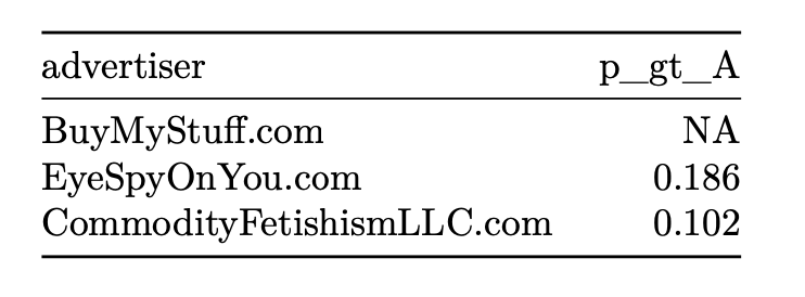
Now we have the probability that each ad, including the one compared against the others, will have the better \(EV\). As you can see these don't sum to 1 so we can't sample from them yet.
This problem is easy to solve by normalizing each value by dividing it by the sum of all the probabilities. If we do that we have this table:

These weighted probabilities become our sampling weights! Let's use this sampling information to select which variant will win the next 500 auctions, then we'll use the information we learned from those to make better decisions in the future!
winners_df <- sample(ad_info$advertiser,
                     prob = ad_info$weighted_p_gt_A,
                     replace = TRUE,
                     size=500) %>%
  table() %>%
  as.data.frame()

ad_info$new_views <- winners_df$Freq
ad_info$new_clicks <- rbinom(c(1,1,1),ad_info$new_views,ad_info$ctr)
Here's what happened showed each ad by its sample weight:

We've now gained some information about how well our unknown ads are doing. Adding in this new information we can update our beliefs...

Even just 500 more impressions changed our belief in how good the CTR for CommodityFetishismLCC is!
Look how much even 500 views has changed our beliefs in each of these ads! With this new info here's how our weights change:

Even after 500 more impression and just one update of our information our Thompson sampling algorithm has already realized that the only two ads really worth focusing on are BuyMyStuff and CommodityFetishismLLC.
Take a moment to realize the value that sampling in proportion to our beliefs has given us. On the one hand had we only used exploitation we would have completely missed out on the opportunity that CommodityFetishismLLC's ad has. On the other hand, if we had sampled uniformly we would have given the ultimately under-performing EyeSpyOnYou too much attention.
One of my personal favorite things about Thompson sampling is that, being fundamentally Bayesian at it's heart, we can understand clearly why we are making every decision we are making. Additionally we can easily inspect exactly what we believe about each ad campaign during our monitoring. Even better is that, because we built this from first principles, there are many extensions we can make: adding more detailed, ad-specific priors, adapting to changing CTRs, dealing with changing bid prices etc.
Continuous updating
We just walked through a single step of Thompson sampling for our Ad auction, but we could continue to do this every 100 impressions. Here is an image that demonstrates our beliefs after running this update every 100 impressions for much longer. There is also a chart showing the sampling weights over time for each variant.

The sampler quickly learns that the only two ads are worth showing, and since they are pretty similar the end up being shown about 50/50
We know that CommondyFetishismLLC is only a hair better than BuyMyStuff so we end up showing them about evenly. Eventually, if we ran this for long enough for our model to detect the very subtle different between the two.
Because our model is constantly learning we have a lot of flexibility with what we can do. This example can scale to a huge number of ads (though we would have to change our computation method for efficiency reasons), and be made to work for a real world ad auction. Additionally we can always add new ads at any time, the model will automatically adjust to explore a new ad that we have less information about. Another interesting option would be to limit the impressions we look at (or weight them by time) to allow for the CTR rate to change. For example, maybe BuyMyStuff’s ad targets summer wear and so have lower CTR as fall approaches.
Conclusion
Thompson Sampling is one of my favor topics to explore because we really get to see the full power of Bayesian reasoning. We have developed a foundation here that takes prior information and parameter estimation to make optimal choices. What’s really fascinating is that we can set this up to be constantly learning about the world dynamically.
While this is a really fun optimization problem, the one caveat I would add to all of this is that very often multi-armed bandit situations can be overkill. What makes the bandit algorithm fascinating, fully automated optimization, is also its weakness. Statistics is best we when it forces us to ask question about and understand better our world, when we turn that to auto-pilot, we can lose more than we gain.
Get source code, behind the scenes commentary and more!

Support my writing on Patreon and gain access to the source code, commentary and pdfs drafts for this article as well as access to much more of my writing!
Keep up to date!
Subscribe for the latest updates to this blog and the current book I’m working on!