There is no shortage of posts on Survivorship Bias out there, so why read yet another one? One problem I realized is that while many articles cover identifying survivorship bias, few discuss how to start thinking about solving these problems. In a time of pandemic and stressful elections it is very helpful to start to think about how we an model problems quantitatively and attempt to correct for biases like survivorship bias. It turns out that identifying this problem is far easier than dealing with it in how we model problems.

In this post we'll be taking a quick look at a real world problem of house hunting during the current pandemic. The pandemic has quickly changed the demand for houses outside of major cities and so many people maybe looking through houses for sale and despairing at their limited options. It turns out that, because of survivorship bias, good homes may be *less rare* than they initially seem.

To solve this we'll model our problem mentally, then mathematically and finally computationally using Python and the JAX library for automatic differentiation. Throughout this process we'll gain insight into what's happening the housing market as well as learning how challenging correcting for bias really is.

Quick Refresher on Suvivorship Bias

Survivorship bias is a common form of logical error where the data that we are presented is representative of only a subset of the population that has already survived a filtering process, meaning that our data lacking important information underestimating the true population that the data comes from.

The classic example of this is the US military looking at the bullet holes in returning bombers during WWII and trying to use this information to determine how to improve the survival rate of planes. The image below illustrates the various location of bullet holes on these planes. The initial reaction of the military was to put armored plates to protect the areas where the bullet holes were on returning planes. When the statistician Abraham Wald was shown this data, he saw this as a clear example of survivorship bias and concluded the opposite: bullet holes on returning bombers indicate where planes could be hit and still survive to fly home. What's missing from this data set are the planes that did not return.

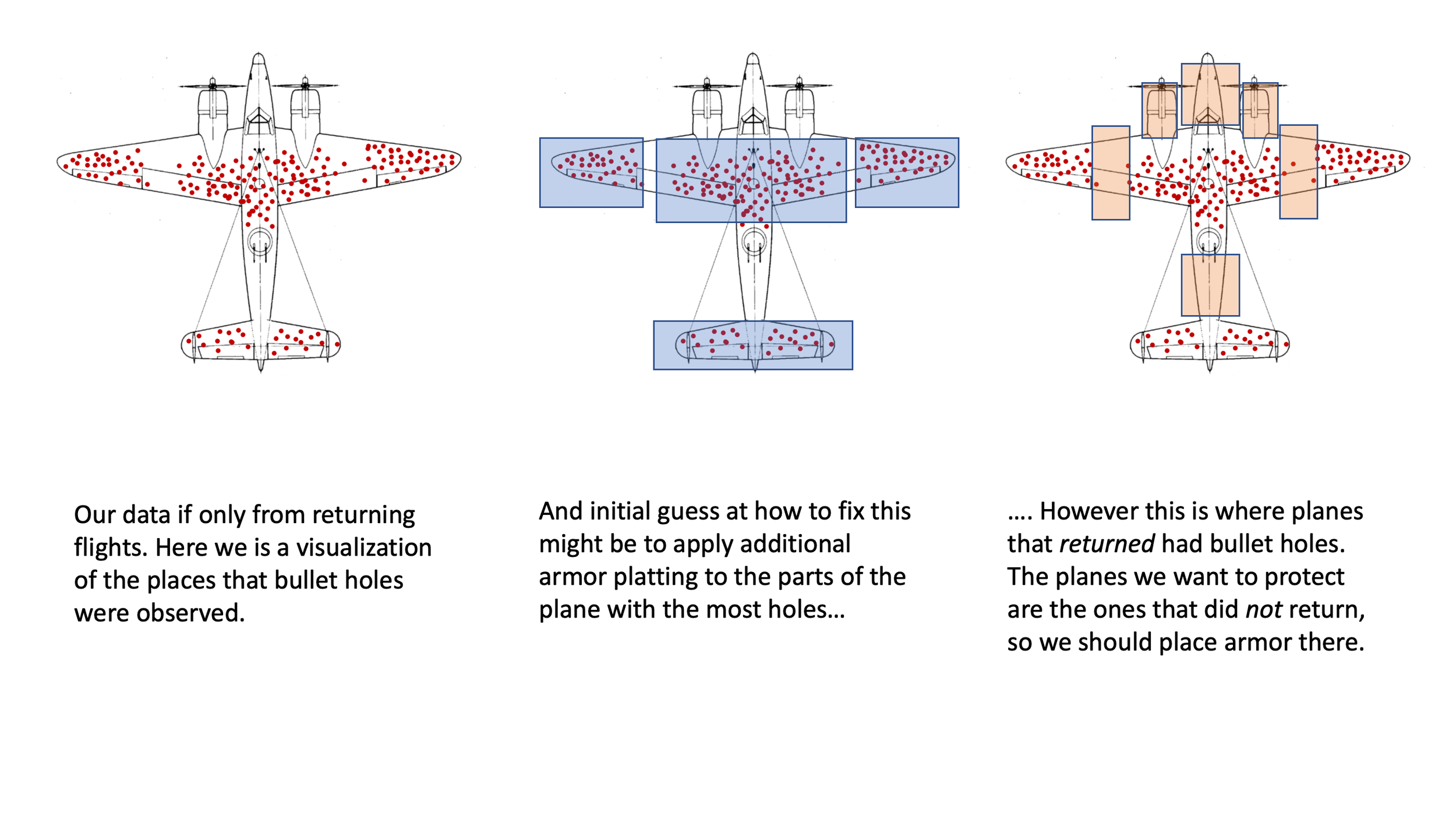
It is legally required to show this image of a plane whenever you write about survivorship bias

The Trouble with Modeling the WWII planes

While the story of the surviving bombers may be a great example of survivorship bias, it doesn't give us much information about how to model and solve this problem.

In this particular example the clever solution requires a large amount of background information about how planes work. For example, seeing that the returning planes have no bullet holes around the engines leads us to immediately conclude that those bombers that did not return were shot in the engine. Since we know how important engines are to the maintenance of planes we can skip over any real mathematical modeling of this problem and use our background information to solve this easily.

But imagine if you were trying to explain this obvious solution to someone that had never heard of an airplane and had no idea how they work, someone who wanted some numerical data to support your beliefs.

The challenge of modeling survivorship bias problems is both very interesting and infrequently discussed, so in this post we'll start to poke at a problem a bit more quantitatively to get a better feel for how to start modeling the this process and how to try to come up with a solution. The main goal is not to solve a problem (because it turns out that really doing that in a satisfactory way is fairly complex) but to start thinking about modeling the problem mentally, mathematically and computationally to have some basic tools for reasoning about a survivorship bias problem quantitatively, if not in a truly statistical manner.

House Hunting in a Pandemic

Like many people living in cities in the US right now, my wife and I have recently started to consider the possibility of purchasing a house in the suburbs outside of the city. Given the rapid shift from office to remote work, and the impact of the pandemic on local city restaurants and bars, it makes a lot of sense of consider moving to a more spacious home for roughly the same price.

Because many people have had this same idea, housing hunting can be an especially daunting, even depressing, experience right now. One of the first steps in the house hunting process is to look at a list of houses currently available from the Multiple Listing Service (MLS) that your realtor gives you access to.

Upon browsing the list of houses my wife and I despaired that of the hundred homes listed, only about 2 of the 100 looked promising. We both have quantiative background and were immediately concerned that going forward we might only expect to find 2% of the homes on the market to be homes we liked. This seemed to be a depressingly low number.

Before despairing too much we both realized that we were facing a survivorship bias problem!

Survivorship bias in the MLS - our mental model

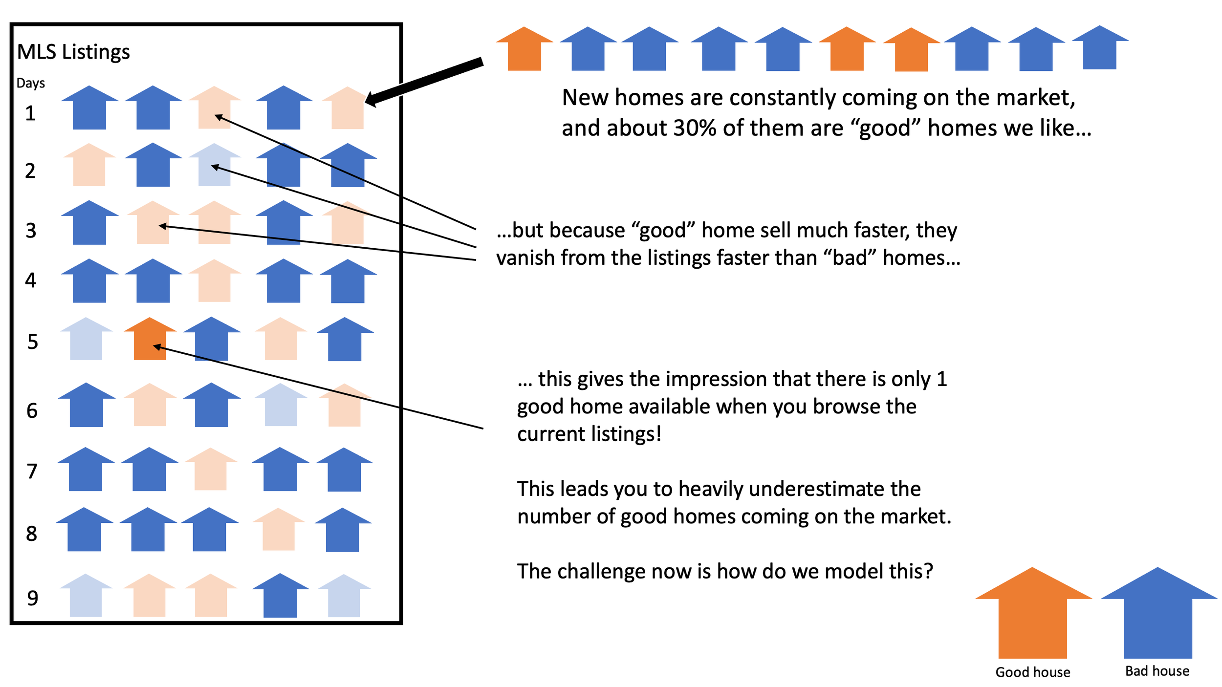
The issue with MLS listings is that these listings might represent houses that have been on the market for up to 90 days. However, we can also assume that good houses will sell much faster than bad houses. This means that if we look at what is still on the market after 90 days the amount of good houses will be much smaller than the amount of bad houses. The question we want to answer is

"how likely are we to see another good house listed next?"

and the number we get from looking at "how many good houses are on the market in listings form the last 90 days" will wildly underestimate the true rate of how many good houses are coming on the market. We can see this visualized here:

The first step in the modeling process is to understand you mental model of how the process works.

We can see that we are dealing with a case of survivorship bias, but noticing the bias doesn't do much to help us solve our problem. What we have here is a mental model of our problem, and what we want is to have mathematical model that will help us answer more specific questions. We know that the observed 2% is much lower than we should expect, but what should we expect? Is it 5%? 10%? as high as 20%? Simply observing that we are experiencing the bias doesn't tell us anything about how we can quantitatively solve this.

Building a “Simple” Mathematical Model of the MLS

To start tackling this problem we need a mathematical model so that we can at least come up with a rough ballpark figure to answer the question:

"What is probability that the next house listed on the market is good?"

For this post we aren't going to truly answer this in a statistical sense since, as we'll discuss later on, there is quite a bit of complexity in really determining our uncertainty. Nonetheless we would like some sort of mathematical model that allows us to get an estimate for the real rate of good houses appearing on the market as well as provides a foundation for building out a more sophisticated statistical model. In practice, when house hunting, you likely don't care particularly about building out full probability distributions of your believes as a much as you are just knowing roughly how much more likely it is to see a good house listed soon based on what you've observed. We'll also see in this post that answering even this "simple" question involves a surprising amount of sophistication.

We want to start by modeling our question itself as parameter and then we can answer our question using parameter estimation. We can imagine that there is some true rate that good houses appear on the market that we can't observe and we only have our listings of the last $N$ days. We'll use the term $\theta_\text{good}$ to represent this rate. In our model $\theta_\text{good}$ is the part of the data generating process the produces the MLS.

Ultimately what we want is to build a model of the MLS listing themselves, of which $\theta_\text{good}$ is only a small part. Once we have this model we can then figure out which is the best $\theta_\text{good}$ for solving our problem. The difference between our

Modeling the Rate the Houses Stay on the Market

A vital part of our mental model is that good houses stay on the market for a shorter period of time than bad houses. What we need to do is figure out a way to model this mathematically. We can imagine good and bad houses being random variables, $X_G$ and $X_B$, that are drawn from two different distributions that describe how long each how will wait until it sells.

It's worth pointing out that this problem by itself could be worthy of a complex modeling process. We could imagine looking at various features of good and bad houses, looking at the day the house is listed etc. But to reduce our complexity we'll just try to find a single distribution that we can imagine each of these being sampled from differing only in the parameterization of that distribution.

At first glance we should be reminded of a Poisson distribution. If we wanted to estimate how many good houses sold in a week, we would use a Poisson distribution to estimate how many events would occur in a given period. However here we want to solve a slightly different problem: how long until an event happens the first time.

For this we can use the Exponential distribution which is used to measure the time between events in a Poisson process.

The Exponential distribution

The Exponential distribution has one parameter $\lambda$ and has the following PDF:

$$exp(x;\lambda) = e\lambda^{-\lambda x}$$

The $\lambda$ parameter represents the rate that an event happens, and the PDF tells us the probability that $x$ is how long we have to wait for an event. For simplicity we'll assume that we know that good houses sell on average every 7 days while bad house sell on average once every 23 days (again, estimating this from data is not as straightforward as we would hope). If we imagine our houses disappearing from the market as individual observations of an exponentially distributed random variable we can imagine something like the following image:

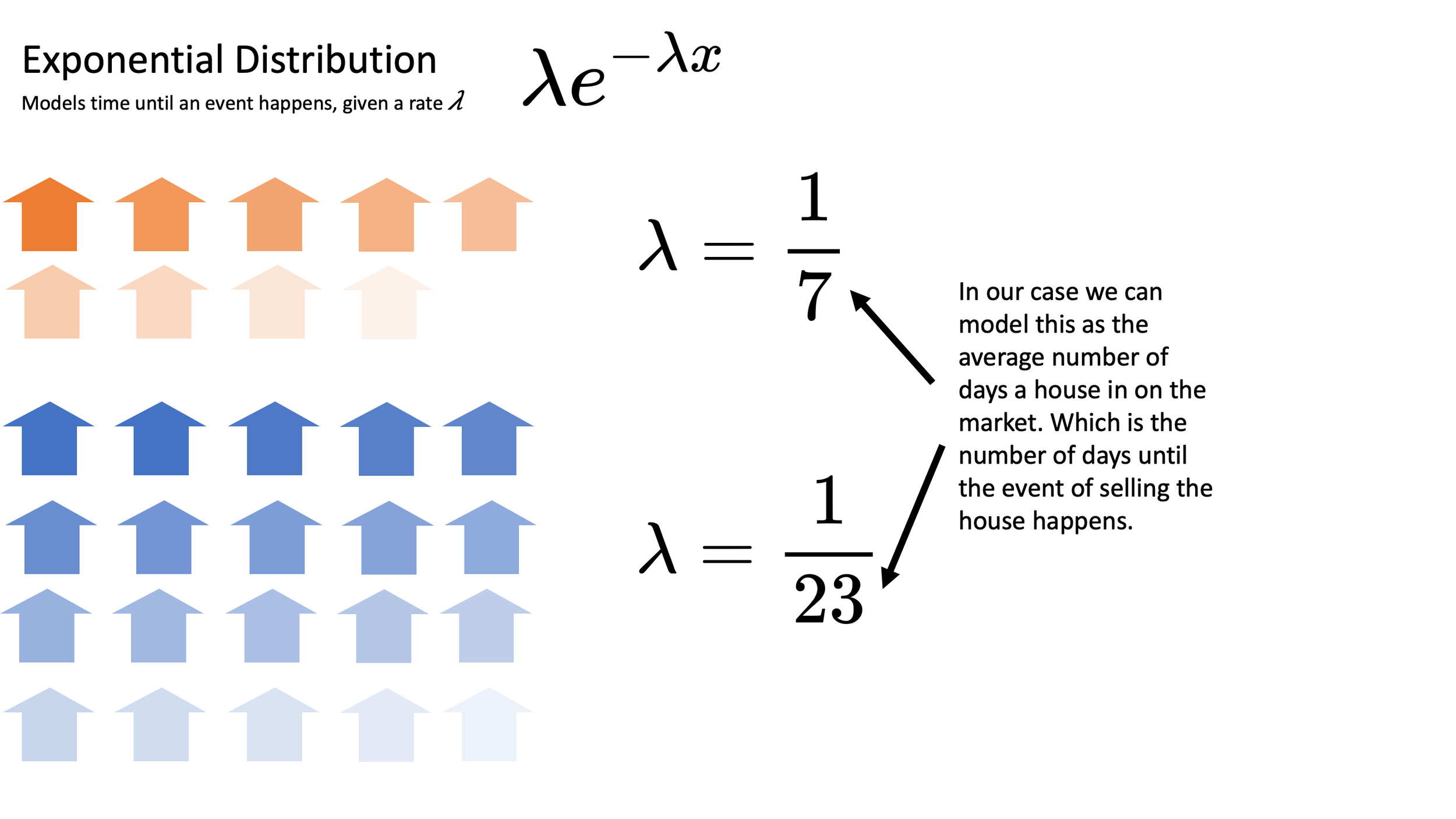
Individual listings can be modeled as observations of an exponentially distributed random variable.

This would allow us to define:

$$\lambda_\text{good} = \frac{1}{7} \text{ and }\lambda_\text{bad} = \frac{1}{23}$$

And we could define our two random variables as:

$$X_G \sim exp(\lambda_\text{good});X_B \sim exp(\lambda_\text{bad})$$

Modeling the ratio of Good to Bad houses on a given day

The MLS postings will have new updates every day and we know that because good houses sell faster than bad houses (at least in our mental model) the ratio of good to bad houses should change on a given day as good houses start to disappear from the listings.

To start with the basics, we can answer "what will that ratio be on the 0th day?". On the 0th day we would expect that ratio to be the probability of having a good house, $\theta_\text{good}$ over the probability of having a bad house, which is the probability of not having a bad house:

$$\frac{\text{good}}{\text{bad}}_{n=0} = \frac{\theta_\text{good}}{(1-\theta_\text{good})}$$

You'll notice that what we have done is really just convert our probability to odds. This will be a useful form to keep this equation in because it will allow us to add together and average the ratios from each day to come up with a model of what the listings will look like with a full $N$ days of observations.

If we next asked the question, "what will the ratio be on the 5th day" we have to edit our formula. We still have the base ratio to consider, but now we have to consider the probability that a house sold, represented by the random variables $X_G$ and $X_B$.

Because we want to compare how many homes are still on the market we don't want to look at the probability that the house sold but that it did not sell. In terms of our random variable, this is the probability that the value of the random variable is greater than the value $n$ for that day. Mathematically we would view this as:

$$\frac{\text{good}}{\text{bad}}_{n=5} = \frac{\theta_\text{good}Pr(X_{G} > n=5)}{(1-\theta_\text{good})Pr(X_{B} > n=5)}$$

This basic formula will give us the ability to calculate each day in the MLS. Next we need to come up with a model for the full MLS that will give us the percent of good houses we would observe given $\theta_\text{good}$, $\lambda_\text{good}$ and $\lambda_\text{bad}$.

Putting it all together

Our listing represent 90 days of observations, which means we need to combine the results of each of these. This solution is pretty straightforward. Assume we just want to add day 0 and day 5. Clearly we can just add these ratios and, assuming we have the same number of listings each day, just average them:

$$\frac{\text{good}}{\text{bad}}_{n=0 + 5} = \frac{\frac{\text{good}}{\text{bad}}_{n=0} + \frac{\text{good}}{\text{bad}}_{n=5}}{2}$$

Note that we are making a pretty bold asymptotic assumption here. We only want to give equal weight to these ratios as the number of houses sold on each day approaches infinity. We're doing this in the name of simplicity, but this is definitely a problem we would want to correct if we were to develop a more rigorous approach to this problem.

We can now extend this logic to get the average ratio of good to bad houses after N days:

$$\frac{\text{good}}{\text{bad}} = \frac{1}{N} \Sigma_{n=1}^{n=N} \frac{\theta_\text{good}Pr(X_{G} > n)}{(1-\theta_\text{good})Pr(X_{B} > n)}$$

Finally we have to fix one small issue. We currently have this in a form that represents the ratio of good over bad, or the odds of seeing a good house in the listings. We want this to be a percentage or probability of seeing a good house. Recall that the formula for converting odds to a probability is:

$$P(H)= \frac{O(H)}{1+O(H)} = 1 - \frac{1}{O(H)}$$

With this formula in hand we can easily transform our odds of a good house into a probability of a good house:

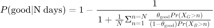
This diagram below visualizes our mental model transformed into a mathematical model:

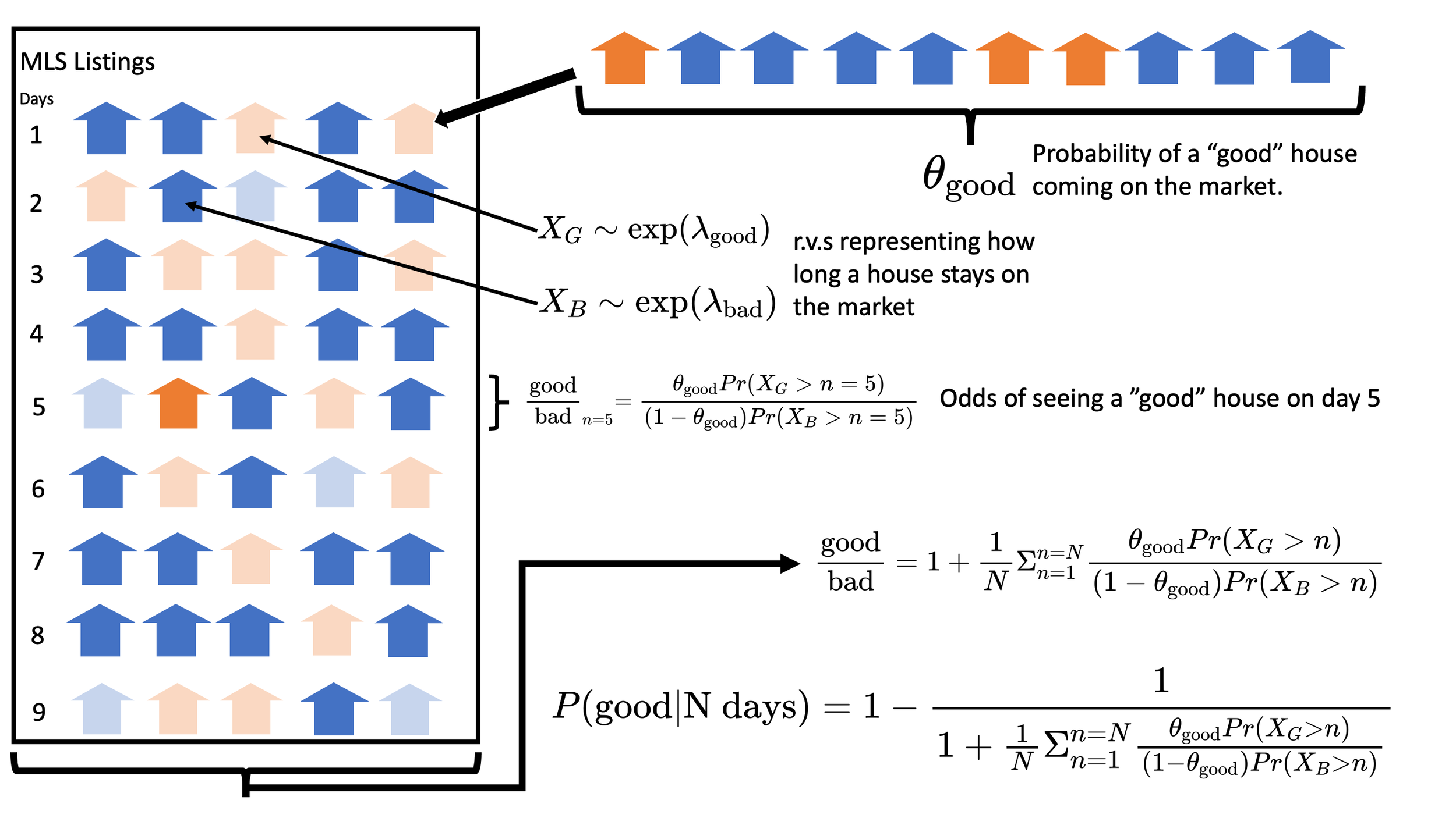
Transforming our mental model into a mathematical one allows us to quantify our beliefs.

Computational Modeling with Python and JAX

We now have a decent first pass at a mathematical model of how the MLS works (which does make some pretty big asymptotic assumptions). Next we need a computational model to solve this problem and we're going to be using Python and the JAX library to help us out. We'll start with importing the few tools from JAX we'll need. JAX is a library that allows us to easily compute the derivatives of any Python code. To help with this JAX has it's own implementation of Numpy. We'll be importing both the JAX version of numpy as well as JAX's grad function we'll use to calculate derivatives.

import jax.numpy as np
from jax import grad

Going back to our original problem let's assume the following:

The listings have 90 days of postings
We see 2% of the houses are good
The average days on the market for a good home is 7
The average days on the market for a bad home is 23

These last two are pretty big assumptions that normally we would have to estimate separately. Fortunately, because we're writing code to solve this problem, we can easily mess around with these to see how sensitive our model is to different values for these. After all our goal here is just to see roughly how likely it is that a good house appears on the market in the coming weeks.

Let's put all of our assumptions in code:

# lambda for good
l_g = 1/7

# lambda for bad
l_b = 1/23

# days in MLS
n_days = 90

# observed probability of a good house
obs_prob = 2/100

Implementing our model

Next we want to create a model of our MLS that we have previously section. I've gone ahead and implemented some pretty straightforward helper functions including exp_cdf which is the cumulative distribution function for the Exponential distribution. This will allow us to easily calculate the probability of a Exponentially distributed random variable taking on a value greater than a given $n$. For example the probability that a good house lasts longer than 10 days is:

1 - exp_cdf(10,l_g)
> DeviceArray(0.23965102, dtype=float32)

I've also implemented to very simple functions to convert from odds to probability, and probability to odds, called odds_to_prob and prob_to_odds respectively.

With these tools we can now implement function to compute the odds that a house is good in the listings given a $\theta_\text{good}$, $\lambda_\text{good}$, $\lambda_\text{bad}$ and $N$.

def odds_good(theta_g,lmbd_g,lmbd_b,N):
    #day 0 ratio is just theta_g
    result = prob_to_odds(theta_g)
    for n in range(1,N+1):
        result += (theta_g*(1-exp_cdf(n,lmbd_g)))/((1-theta_g)*(1-exp_cdf(n,lmbd_b)))
    return result * 1/N

Without much work we were able to transform our mathematical model into a computational model. The next step for us it so use this to solve our actual problem, which is determining what the value for $\theta_\text{good}$ should be given our assumptions.

Newton's Method and Root Solving

To start off we need some way to assess how good a given guess for $\theta_\text{good}$ is. An obvious way is to just measure the difference between the probability of good given the model parameters and the observed probability of good houses. Here is our `target` function that does precisely this:

def target_func(target,theta_g,lmbd_g,lmbd_b,N):
    return target - odds_to_prob(odds_good(theta_g,lmbd_g,lmbd_b,N))

If we know the values of target, lmbd_g, lmbd_b and N then we can think of this problem as trying to find the root of this new target function with respect to theta_g. The root of a function is the value of the argument where the result of the function is 0.

The classic way of finding the root of a function is Newton's Method. Newton's method is an iterative method that continually updates a guess $x$ by using the derivative of the function. The traditional update rule for Newton's method is:

$$x_{t+1} = x_{t} - \frac{f(x_t)}{f'(x_t)}$$

All we have to do now is find the derivative of our target function!

Using JAX to calculate the derivative

In order to appreciate how nice it is to have JAX, let's take a look at what our target function, which we'll just call $f$, looks like in full with all of our parameters in place:

$$f(x) = 0.02 - (1-\frac{1}{1+\frac{1}{90} \Sigma_{n=1}^{n=90} \frac{x(-e^{-\frac{1}{7}n})}{(1-x)( -e^{-\frac{1}{23}n})}})$$

If you want you can go ahead and work out the derivative of that by hand (or with Wolfram Alpha), but I'm going to take the JAX approach and just use grad. This following bit of JAX will automatically compute this derivative for us:

d_tf_wrt_theta_g = grad(target_func,argnums=1)

In fact this JAX code is even a bit better since it's computed the partial derivative with respect to the argument in position 1 (zero-index) which means I can still parameterize this function with what ever other values I want for the other parameters I'm assuming.

From here solving our problem is reduced to iteratively implementing Newton's method. We'll go for just 5 iterations, but could easily change that based on the stability of our answer:

guess = 0.5
iters = 5
for _ in range(iters):
    f_val = target_func(obs_prob,guess,l_g,l_b,n_days)
    df_val = d_tf_wrt_theta_g(obs_prob,guess,l_g,l_b,n_days)
    guess -= f_val/df_val
print(guess)
> 0.14804904

In the end, based on our simple model, we should expect that about 15% of the new houses coming on the market will be good, rather than the observed 2%. This really goes quite a ways in reducing our despair!

Is our model too simple?

One thing should be very clear at this point in the process: modeling for survivorship bias is wildly more difficult than correctly identifying it. The purpose of this post was to get us to start seeing how challenging that process is. At this point we have a rough sense that, given the many assumptions we are making, observing that 2% of the houses in the listings are good, accounting for survivorship bias, we should not despair as the rate good houses come on the market should be much higher.

However, other than feeling a bit better about house hunting, we have ignored a profound amount of information. Most important of all we do not have a statistical model of the MLS. We are able to derive the best guess, but right now we have absolutely no idea how to say how good that guess is. Is it possible that 20% of the houses are really good? What about 50%? In order to come up with a probabilistic model we want to solve our problem in the form of:

$$P(D|\theta_\text{good})$$

That is we want to answer the question "how likely are the MLS results we observed, given our belief in as specific $\theta_\text{good}$". Our work so far should provide some guide to how to get there, but we are still a long way from the correct solution.

This is also ignoring many of the other caveats that were noted throughout our modeling process. Just estimating our $lambda$ values is going to be challenging since these too are subject survivorship bias. So even this "simple" model contains an enormous amount of complexity in modeling. This doesn't even begin to consider that maybe our basic worldview of only "good" and "bad" houses might be overly simplistic, or that the housing market behavior might change over time.

Sympathy for election forecasters

Survivorship bias is just one of many forms of bias that exist. At the time of this writing, results from the 2020 US Presidential election are still being counted and many people (myself included) are voicing their frustration with election forecasters. But I do hope that this post helps to generate some sympathy for anyone trying to tackle this problem. Election forecasters must combine vastly larger amounts of information than we see here. Additionally that data, largely from polls, is subject to a wide arrange of different biases. All of this to predict the outcome of an event that is hard to determine the result of when the data itself is present! We have a huge percentage of the votes recorded at this moment, and still don’t know officially who has one the election.

Along with sympathy for the forecasters I also recommend a hearty skepticism of the forecasts. I would argue that the most important part of the modeling isn't the prediction, but the process. Looking at forecasts for a point estimate of who will win or lose is of very limited use. Looking at the data that feeds into those forecasts, thinking about how you would quantitatively adjust for different biases, and building a model for how the world works are all tremendously insightful pieces of the processes. Being right in statistics is not nearly as important as knowing when you are surprised, what surprises you and how that should change your beliefs.

In our real estate example, suppose in the coming weeks we still saw very few good houses. Because of this model we can start asking why that is? Do "bad" houses leave the market much faster than we thought? Is the market changing as the pandemic develops? Having a model in place allows us to ask these types of questions and start thinking how we might investigate answering them quantitatively.

Get source code, behind the scenes commentary and more!

Support my writing on Patreon and gain access to the source code, commentary and pdfs drafts for this article as well as access to much more of my writing!