This post is the first in a three part series covering the difference between prediction and inference in modeling data. Through this process we will also explore the differences between Machine Learning and Statistics. In my career as a data scientist I've found that there is a surprisingly lack of understanding of the task of inference which is typically considered the domain of statistics. Though it is less common, I have also found that people I know well versed in statistics often have a tough time understanding the way machine learning thinks about prediction tasks.

A little over a year ago I posted an image to Twitter summarize my views on this distinction visually:

In the series we’ll ultimately see who these two are more connected than they are typically treated

In this post I want to not only flesh this idea out through a worked example, but also attempt to blur that distinction. Ultimately the aim of any quantitative thinker should be to see modeling as a holistic process that extends our mathematical reasoning to its fullest. Especially in an age of easy computation, the process of modeling should be a highly interactive one that extends beyond the synthesis of these two ideas.

Our Example Problem: Modeling Click Through Rate

One of the most common problems in industry is modeling Click Through Rate (CTR). Generally CTR problems show up whenever we care about a user performing some task, usually 'clicking' on some piece of content. Common CTR problems include: a user signing up for a service via a form, clicking on an ad, looking at an item description in a catalog, purchasing that item, reading a post on an new aggregator, etc.

In a previous post we talked about the process of Thompson Sampling to optimize an ad auction . One of the key parts of this article was estimating the CTR using the Beta Distribution with only data about previous clicks per view. While this approach worked great for that example we often have a lot more information at hand that we would like to use to better understand when a user will click.

In this example we'll be using information about the CTR for job postings on a job board. The data is derived from this Kaggle data set. Using this data set we are going to attempt to learn whether or not a user will apply for a job given we know information about what category that job is in, and how similar various parts of the job title are to the user’s original search query.

In my career in data science I have been shocked by the number of time that CTR problems are treated as pure prediction problems. As we will see in this post, treating CTR as a prediction problem leads to a limited view of how to solve various common problems related to CTR (namely how do we improve it!). To start we'll treat this problem from the perspective of Machine Learning, building a simple perceptron model from scratch using Python and JAX and then, in the next part, learn how we can naturally extend this model to cover inference.

A look at our data

Before we begin here's a look at the cleaned up version of our data set. We have the following features we'll be using:

features = ['main_query_tfidf', 'query_jl_score',
            'query_title_score','job_age_days',
            'job_16140', 'job_31542','job_41757',
            'job_42467','job_45300','job_51966',
            'job_67237', 'job_69982', 'job_77312',
            'job_82238','job_other']

The first 3 features correspond to various similarity scores between the query text and the job posting text, then we have the number of days the job has been on the board, and finally we have the top 10 job category codes and an indicator if the posting was in another category.

Here is a peek at what this data looks like, mean centered, and with the standard deviation normalized:

apply_data[features]

As you can see at the bottom we have plenty of data with 1,200,890 rows.

For the rest of this post we'll mainly be doing lots of computation so we'll be transforming this data into a jax.numpy matrix and splitting it into test and training sets.

import jax.numpy as jnp

X = jnp.array(apply_data[features].values)
y = jnp.array(apply_data['apply'].values)

train_size = int(np.round(0.7*float(X.shape[0])))
indices = np.random.permutation(X.shape[0])
X_train, X_test = X[0:train_size], X[train_size:]
y_train, y_test = y[0:train_size], y[train_size:]

With that out of the way we can begin our modeling!

Prediction - The Machine Learning world view

Now that we've finally cleaned up our data it's time to start modeling! If you're an experienced data scientist or machine learning engineer, then much of this article will be very familiar to you. That is intentional because I want to show the logic that connects a very traditional machine learning world view with a statistical one. So even if this is a familiar topic, it's worth reiterating how we think about solving machine learning problems.

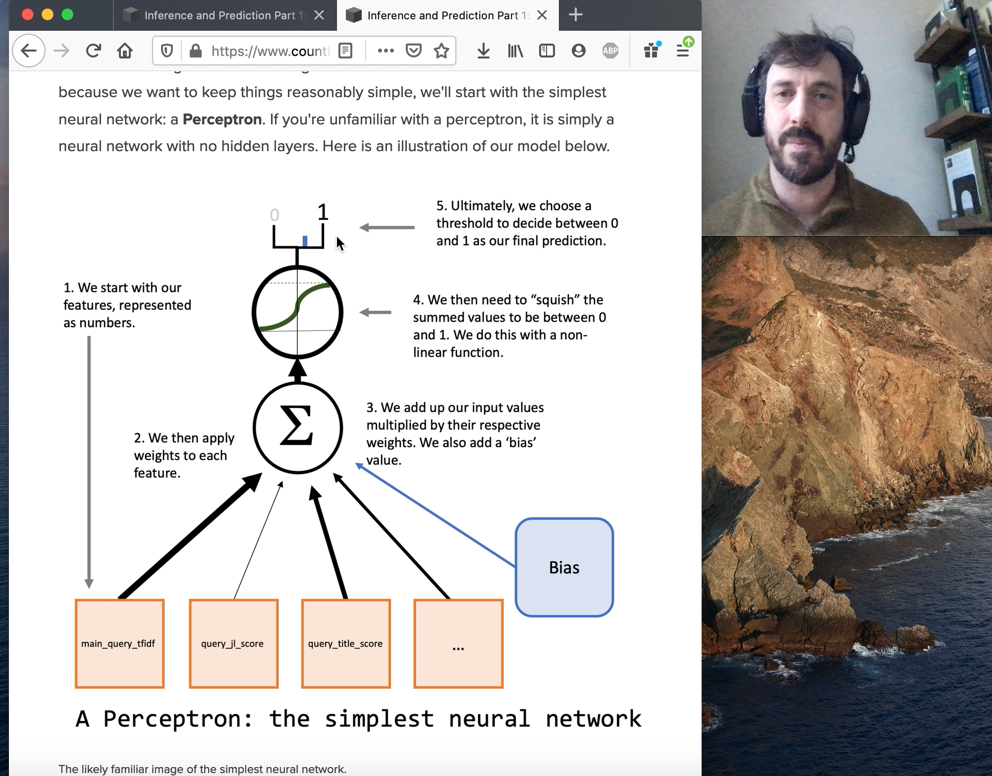
Since we're doing Machine Learning we'll want to start with a neural network. But because we want to keep things reasonably simple, we'll start with the simplest neural network: a Perceptron. If you're unfamiliar with a perceptron, it is simply a neural network with no hidden layers. Here is an illustration of our model below.

The likely familiar image of the simplest neural network.

Note that there is a "bias" node in that visualization of our how model will work. We can represent this this by simply adding a constant to our data, which I've already gone ahead and added to our X_train and X_test sets.

Putting together our model

Let's start thinking about our problem mathematically. We have a picture of what our perceptron looks like, but we want to figure out how to make this happen. We have $X$ and $y$ which is our data and our target respectively. We now have a couple of things we need to add.

The first step is to represent all of those lines in the network diagram numerically. We'll do this with a vector of weights $w$. What should the value of those weights be? Well, we are going to have to learn that (or actually we want the Machine to learn that).

We're going to use JAX again here, and we'll be using it to create random weights. Unlike standard Numpy, JAX always needs a key in order to create random values. This means that our random variables are always predictable. This is very convenient for debugging our model since even though we will be doing many random actions, they can always be repeated exactly. Here is an example of how we will create a vector of random weights:

from jax import random
key = random.PRNGKey(1337)
w = random.uniform(key, 
                   shape=(X_train.shape[1],), 
                   minval=-0.1,
                   maxval=0.1)

The lines in the illustration represent us multiplying the values in our data by the weights and summing them up. Mathematically we can represent multiplying the inputs by the weights and summing them up quite simply using linear algebra:

$$Xw$$

Here we can see using this in code:

jnp.dot(X_train,w)
> DeviceArray([0.15793219, 0.07844558, 0.07844558, ..., 0.27550998,
             0.10248479, 0.13946426], dtype=float32)

We're not done with our model yet. There is an obvious problem already. We want to predict 1 (for will apply) or 0 (for will not apply), but we need a way to ensure that our predictions are always somewhere in this range. In order to solve this problem we need a non-linear function that will squish our values between 0 and 1. Using $g$ to represent a non-linear function, we can now look at our full perceptron model mathematically as:

$$y = g(Xw)$$

Our choice for $g$ will be the logistic function, which has the nice property of squishing values between 0 and 1. It also has the very nice property that it allows us to model our predictions as probabilities. We'll touch on this again in part 2, but it's important to recognize for when we want to train our model. Here is the logistic function mathematically:

$$g(x) = \frac{1}{1+ e^{-x}}$$

Here is the logistic function in code:

def logistic(val):
    return 1/(1+jnp.exp(-val))

We can apply this to X and our random weights and we can see we have our first model!

guesses = logistic(jnp.dot(X_train,w))
guesses
> DeviceArray([0.5394012 , 0.51960135, 0.51960135, ..., 0.5684451 ,
             0.52559876, 0.53480965], dtype=float32)

These are, in a very literal sense, random guesses. The next step is to figure out how we can improve them.

The "learning" part of Machine Learning

Of course our model doesn't know anything about the world. We can see that all of these initial guesses are pretty close to 0.5, right in the middle of our choices of 0 and 1. When we make a prediction we commonly choose (or, more commonly, software chooses for us) 0.5 as the threshold between choosing 1 or 0. If we did that now we would find that our guesses would roughly estimate that half the cases would be apply and half not. They can be slightly skewed because of the distribution of the values in X, but otherwise we’re just multiplying uniformly distributed numbers (our weights) by values that we’ve transformed to have an expectation of 0 and standard deviation of 1. When we do the logistic transform of 0 we get 0.5, so most of our initial guesses will be pretty close to 0.5. Clearly we need to improve what our weights are from random guess to ones that best map our data to the correct result.

People like to joke about the term "Machine Learning" for simple cases like this, but it really is a pretty good description of what is about to happen. We want the machine (i.e. our computer) to learn the best $w$ for this model. The key to this is figuring out some way to let the machine know whether or not one guess at the weights is better than another one. We’ll do this be creating an objective function (often known as a loss function) that let’s the computer know how good its attempts to improve the model are.

We mentioned earlier that one of the benefits of using the logistic function is that we can interpret the results as probabilities. That is a 0.2 means that's a 20% chance that a a user will apply for a job, and 0.75 means there's a 75% chance that they will. Our labels still work since we can interpret them as being 0, for we know they did no apply and 1 it's absolutely a fact that they did.

This gives an intuition about how we can set up our objective function that we want to optimize. If our model predicts 0.75 and the result is 1, can ask ourselves:

"What is the probability that we would get a 1 if we thought the probability of a 1 happening was 0.75?"

Clearly this is just 0.75. As a counter example, if our model says 0.75 and we get 0, the probability of that happening if our model was correct is just 0.25. That is what we want is a function to tell us how likely the outcomes are given a set of weights. Once we have this then we just need to find weights that are most likely to explain the data. This is the Maximum Likelihood approach to finding the best weights.

The Reasoning Behind Negative Log Likelihood

We've just looked at determining the likelihood of a single point of data, but we want to figure this out for the entire 840,623 rows in our training set. Here is some code that will compute the likelihood of the data given the weights for the entire training set (p_d_h stands for Probability of Data given the Hypothesis $P(D|H)$).

y_prob = logistic(jnp.dot(X_train,w))
p_d_h = jnp.where(y_train == 1, y_prob, 1-y_prob)
print(p_d_h)
> [0.46059883 0.48039865 0.51960135 ... 0.4315549  0.47440124 0.46519035]

Each of these observations represents how likely the outcome we observed would be if our model was correct.

What we want to do is combine all of these in to a single likelihood of the data we observed given the model we have. To do this we can just take the product of all of these:

$$P(\mathbf{y}|Xw) = \prod_{i=1}^N P(y_i|Xw)$$

This represents the joint probability of all of these observations if we assume our model is correct.

While this is mathematically correct we can quickly see a problem with this approach:

jnp.prod(p_d_h)
> DeviceArray(0., dtype=float32)

Because we are taking the product of over 800,000 probabilities, this number is smaller than the lower bound of what we can represent on a computer. The probability of our random guess is zero, but even the probability of nearly prefect guesses, say ones with a 0.99 probability, would be:

$$0.99^{840,623}$$

Which will still be zero on a computer.

A great solution to this problem is to convert our probabilities to log form and take the sum of them rather than the product. This will give us the log likelihood which is much more practical when we're using a computer. As you can see the log likelihood is much more stable of a number:

jnp.sum(jnp.log(p_d_h))
> DeviceArray(-619300.56, dtype=float32)

There is one final issue we'll have with this result. Generally optimization techniques are designed to find the lowest value of a convex function. For log likelihood the smaller the number, the lower the likelihood, which is the opposite of what we want. Thankfully, since our log likelihood will always be less than zero (since our likelihood itself is always less than 1), we can take the negative log likelihood and end up with a nice, convex function we can put together.

Here is all of that put into a single function:

def neg_log_likelihood(y,X,w):
    y_prob = logistic(jnp.dot(X,w))
    p_d_h = jnp.where(y == 1, y_prob, 1-y_prob)
    ll = jnp.sum(jnp.log(p_d_h))
    return -ll

And now we can see what the negative log likelihood of our data given our weights is right now, before we learn anything:

neg_log_likelihood(y_train,X_train,w)
> DeviceArray(619300.56, dtype=float32)

As you can see the negative log likelihood is a positive number (since all log numbers between 0 and 1 are negative). What we want to do now is find values for $w$ that decrease this number and thereby ultimately increase the probability of our labels given the weights.

Optimization - Good 'ol Gradient Descent

Our machine is almost ready to learn! One helpful way to think of the $w$ is as being a specific definition of a model. With negative log likelihood we now have a way to say when one model is better than another, and it is specifically when this value is lower.

What we have here is a traditional optimization problem: we just need to systematically lower the negative log likelihood until we find a place we think is the lowest. We'll be using gradient descent which allows us to use the derivative of our objective function to help us find the lowest point.

So the only problem we have left is to find the derivative of this negative log likelihood function. Historically getting the gradient was a bit annoying since you had to calculate the derivative by hand. The true power of JAX is it will automatically solve that problem for us, making this operation trivial in code:

from jax import grad
d_nll_wrt_w = grad(neg_log_likelihood,argnums=2)

In this call to grad we are determining the derivative of the negative_log_likelihood with respect to the argument in the 2 (zero indexed) position, which is $w$.

Next we'll put together a quick version of gradient descent. Given the decade long frenzy over neural networks there are countless tutorials on the details of this so we won't spend much time covering them. The basic idea is that we use the derivative of our loss function to slide downhill until we find our optimum.

One step we'll add is compiling our gradient function so that it runs more efficiently

from jax import jit
d_nll_wrt_w_c = jit(d_nll_wrt_w)

Since we're approaching this optimization problem pretty casually we can just manually run this a few times until the negative log likelihood looks like it converges.

lr = 0.00001
for _ in range(1,200):
    w -= lr*d_nll_wrt_w_c(y_train,X_train,w)

print(neg_log_likelihood(y_train,X_train,w))
> 251421.27

Now we have trained our model! The next step is to see how well it does at modeling the rates users apply to job listings.

Statisticians: "But wait isn't that really just..."

I want to make a quick aside to address a frequent misunderstanding that I see from people in the statistics community. Statisticians will immediately recognize that our specific implementation of a perceptron is going to be equivalent to logistic regression (something we'll explore more in part 2). A frequent criticism from statisticians is:

Is this really machine learning? It's just Logistic Regression which I use everyday without thinking about it!

I would argue that the important distinction is precisely that Machine Learning practitioners do think about it. That is, the optimization process, choosing a loss function to optimize, choosing a method of optimization, is an essential part of the modeling process. For example, for traditional linear regression the statistician will almost always just default to Ordinary Least Squares regression. This is akin to choosing Mean Squared Error as the objective function, which changes what we can do with our model as opposed to if we had chosen negative log likelihood.

As model complexity increases in Machine Learning questions around objective functions and the optimization techniques themselves take center stage. But even in this simple case I chose negative log-likelihood for a very specific reason, even though there are many options to learn essentially the same $w$. In both parts 2 and 3 negative log-likelihood will allow us build extensions to our model with a trivial amount of code.

We are seeing statistics change in this regard. Nearly all work in cutting edge Bayesian inference requires a deep understanding of optimization techniques and numerical methods. Traditionally speaking, this focus on computation and the details of optimization is a key distinguishes between the worlds of machine learning and statistics.

Measure the Performance of Machine Learning Models

It's good to take a moment here to think about what we are trying to measure as far as gauging the success of our model. Ultimately, in machine learning we are trying to predict something. Right now the output of our model is going to be a number between 0 and 1, these are the model's predictions.

Our model can also be considered a classifier. We are thinking of the model ultimately making a prediction about whether or not the user represented in the data will apply for the job or not. In the process of building a classifier we are going to have one final transformation in our model which is to decide whether or not to return a 0 or a 1 as our final output.

There are a variety of metrics that can be used to assess this task. When we ultimately want a classifier it's intuitive to immediately turn towards accuracy, the ratio of correct to all guesses, as a first measure. However, there are two problems with accuracy. The first is apparent when we look at the proportion of applies to total views in our data:

sum(y_train)/y_train.shape[0]
> 0.0899083179974852

So we have the classic problem where of an imbalanced data set (though, I think that's a bit of an odd way to think about it, especially we're modeling a rate). The real issue here is that just guessing 0 for everything would yield us a very impressive accuracy.

The other, more subtle problem, is that we really haven't thought much about when we choose 1 or 0. In nearly every machine learning library this choice is quietly made for us at 0.5. This nearly always configurable, but I've received many perplexed stares when asking data scientists "what is the threshold your model is using to predict 1?" We could more formally describe this choice as as minimal soft max layer in a neural network.

But we don't really know what a good point would be to call it in favor of a user applying, so we will use a metric that sees how good our model will perform at varying thresholds: The ROC AUC (a metric that deserves a post on it's own one day).

If you're unfamiliar, ROC AUC look at the area under the curve based on the change in true positive and false positive rates at various thresholds. In general an AUC of 0.5 means we are essentially guessing as far as classification goes and 1.0 is the perfect classifier.

Let's take a look at calculating this metric for the training and test set:

from sklearn import metrics
pred_train = logistic(np.dot(X_train,w))
fpr, tpr, thresholds = metrics.roc_curve(y_train, pred_train)
metrics.auc(fpr, tpr)
> 0.5758443732443408

pred_test = logistic(np.dot(X_test,w))
fpr, tpr, thresholds = metrics.roc_curve(y_test, pred_test)
metrics.auc(fpr, tpr)
> 0.5751280457175497

This is not good. This AUC means that our classifier is not able to effectively discriminate between people who will apply and those who will not. From this perspective, it looks like our model is a failure.

The Limits of Machine Learning

But did our really model fail? For starters, let's take a look at what we learned. Our final log likelihood was -251,422 and our initial was -619,300. Recall that:

$$\frac{A}{B} = e^{log(A) - log(B)}$$

Which means that we improved our initial likelihood by a factor of:

$$e^{366,878}$$

After all the work our model explains the data better by such a large amount that we can't represent that value on a computer! So we did do a lot of learning.

The real issue is that we are misunderstanding how to judge our model. Accuracy, AUC, Precision, Recall, F1 Score etc are all common metrics to measure the performance of a classifier. However from the beginning we have said that we are modeling the Click Through Rate. Whenever we've tried to measure rates in the past we often have used statistics to come up with distributions of beliefs about what that rate could be.

Misunderstanding modeling Rate problems as Classification problems is one of the most ubiquitous modeling errors I have seen in industry. A super human, perfect model of a rate will often be a bad classifier.

A great example of this is modeling a coin toss. If we have a fair coin, and your model says the rate of flipping heads is exactly 0.5 with no uncertainty, then you have a perfect model of how the coin behaves. However if you treat this rate model as a classifier it will have abysmal performance. Similarly suppose you are playing some lottery where the big prize has a 1/1,000,000 probability of paying out. Again, if you have a model that, with no uncertainty, predicts the exactly probability of a win at 1/1,000,000 you have the perfect rate model. This will also be an awful classifier.

Even if these rate models don't work as classifiers the can be essential for properly making decisions under uncertainty. Without a correct model of the coin we can make incorrect assumption about whether we should bet $1 for a coin toss where the winner gets $2.1 if the coin lands heads.

The problem of prediction

But the problem goes deeper than just misunderstanding modeling rate problems for modeling classification problems. After all, we could consider the output from the model before we threshold the prediction. Then we could try to come up with some metric that might better assess this result.

Even with that adjustment though, ultimately what our model is giving us is a single prediction, a point estimate, of what the rate is given the information we have. Any frequent readers of this blog will immediately ask the question "how sure are we of this estimate?" This is especially important if we are going to do things like optimizing ad auctions, or any expected reward given uncertain risk. To answer this question we need Statistical Inference.

In the turn to statistical inference we will start to pay closer attention to what the model actually learned. This is essential because the 'rate' doesn't implicitly exist in the data in the first place, it's a part of our model. To understand rate problems correctly, we need to understand the model itself and not just its output.

For that we need statistical inference.

Coming up next: Statistical Inference

In the next part of this series we'll approach statistic inference from exactly where we left off. This will show us how deeply connected the ideas of Machine Learning are with Statistical Inference. In part 3 we'll explore how Inference and Prediction are both parts of a single modeling process, one that transcends thinking about problems in purely statistic, or purely machine learning terms.

Get source code, behind the scenes commentary and more!

Support my writing on Patreon and gain access to the source code and video commentary for this article as well as access to much more of my writing!