As a writer, I’m frequently disappointed with the quality, and in particularly the feel, of LLM writing. For many practical purposes it is, of course, perfectly passable, but I think we all instantly get that “oh, an LLM wrote this” vibe when we read writing from an LLM. Now as an AI engineer, I feel like this must be a problem we can solve! In this post I attempt to solve this by modifying the sampling process for an LLM by incorporating information about the future entropy (related to the diversity of choices in the next token) that the model has given it selects a particular token.

There’s fairly interesting clip circulating social media of Ben Affleck discussing the role of AI in writing that expresses this problem with LLM writing quite well:

“If you try to get [AI] to write you something it’s really shitty. And it’s shitty because by its nature it goes to the mean, to the average.”

— Ben Affleck

What is interesting about Affleck’s point is that he seems to correctly identify the problem (AI writing does tend to be shitty) and gets surprisingly close to correctly guessing the problem. Affleck recognizes that in a sense LLMs are “going to the average” in that traditional LLMs are trained to basically optimize the expected next token.

It turns out though, we have much more control over the LLM’s behavior (especially when working with local models), and by performing our own customization regarding how LLMs generates text we can improve the quality of the result!

Understanding the Role of Sampling in an LLM

Before we go further it's worthwhile to briefly revisit the mechanics of the final stages of the process of an LLM generating tokens. Below we have a diagram of how LLMs generate tokens are we’re going to be particularly interested in steps 4 (logits) and 5 ( sampler) in the image below:

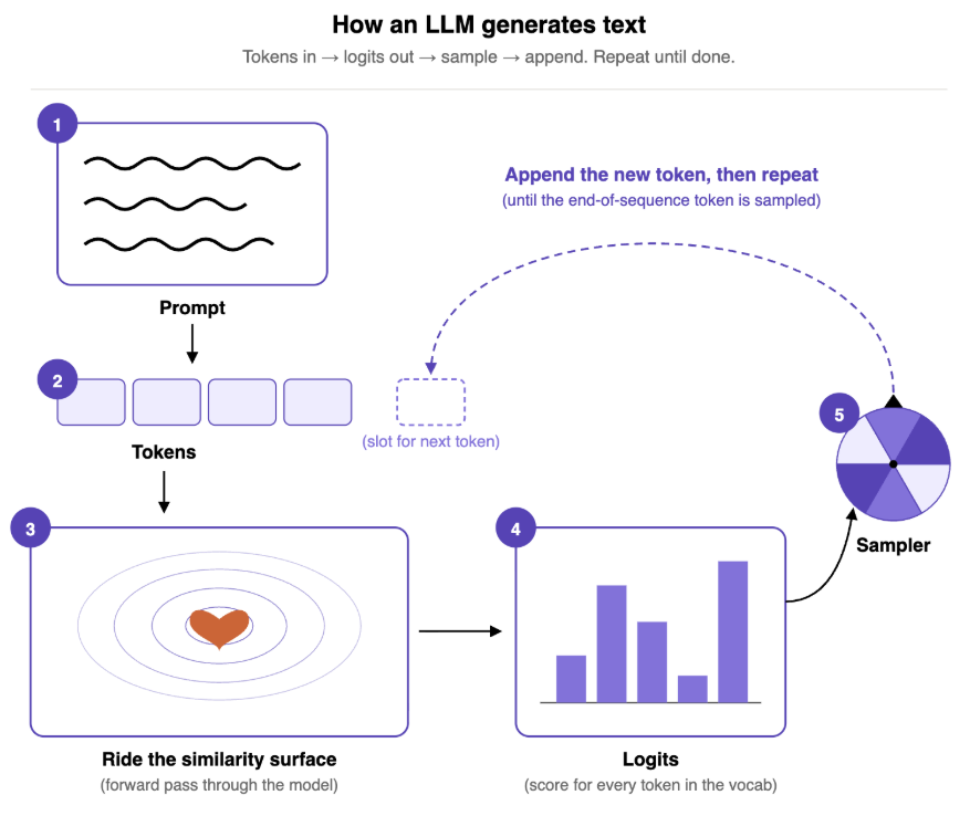
Diagram of how an LLM generates text, we’re concerned with steps 4 and 5, the “similarity surface” is a talk for another post!

All of the incredible work that an LLM does ends up in the logits which can be easily transformed into a probability distribution over the vocabulary next tokens $V$ given the previous context $c$ (i.e. the prompt): $\text{p}(V \mid c)$. “How likely is each next token?” is essentially what the logits tell us, but what they don’t tell us is how to choose!

This is the job of the sampler! The sampler is basically our strategy for how to pick the next token ($w$ in notation) and it plays an incredibly important role on what the output of an LLM actually looks like. To understand this better, let’s take a look at two common samplers we’ll be using in this post.

Greedy Sampling

The easiest sampler to understand is the greedy sampler. The greedy sampler simply chooses whichever token has the highest probability a each step in the generation process. Mathematically the greedy sampler is defined as:

$$w = \arg\max_{v \in V}\ \text{p}(v \mid c)$$

Interestingly enough, the results of greedy sampling are consistent and predicable. Most people talk a lot about LLMs being stochastic (some people say “non-deterministic” but that word has a much more interesting and specific meaning in computer science), however being stochastic is not a fundamental property of the transformer architecture, but rather a property of the sampler. If you run the same prompt through an LLM using a greedy sampler you will get the same result!

Greedy samplers tend to create very boring results (as we’ll see soon), but are useful for things like solving math problems or answering fact based questions where we don’t want the model getting too creative.

Temperature based sampling

Most users of proprietary LLMs are familiar with the concept of temperature when using an LLM. Temperature often is associated with how creative one wants the model to be. Since we’re interested in LLM creativity its worth defining precisely what temperature based sampling is.

When we’re not doing greedy sampling we often want to simply select the next token by sampling based on its probability (typical of how we often approach sampling from any known distribution). For example if a token has \p(v \mid c) = 0.25 \) then we have a 25% chance of choosing that token. The idea of temperature based sampling is that we can supply a number, $T$ from 0.0 to 2.0 that adjusts the shape of that distribution. Choosing 0.0 is effectively the same as greedy sampling, 1.0 is the natural distribution (leading to a 25% chance as in our last example) and 2.0 squishes the distribution close to every token being equally probable.

More formally: Temperature $T$ rescales the logits before turning them into probabilities, then samples from the distribution:

$$\text{p}_T(v \mid c) = \frac{\exp\!\big(z(v \mid c)/T\big)}{\sum_{u \in V}\exp\!\big(z(u \mid c)/T\big)}, \qquad w \sim \text{p}_T(V \mid c).$$

Generally $T=1.0$ is recommended as the choice for “creative” results when working with models when temperature sampling ($T=2.0$ tends to be too extreme in practice to get anything coherent).

Creating new samplers

One thing that has often fascinated me is that in the generative image AI community, choosing and even creating your own custom sampler is a major part of the workflow. My upcoming book on generative image AI, Beyond Slop, has an entire chapter devoted to how to use and choose samplers! But for some reason, in the LLM world we tend to at most tweak the temperature.

We’ll break this pattern by building out a sampler of our own! First we need to learn a bit more about an essential concept for this sampler: entropy

Entropy and Normalized Entropy

Without of doubt entropy is one of my favorite concepts in probability and information theory. Originally introduced in Claude Shannon’s excellent A Mathematical Theory of Computation entropy is commonly understood as a measure of information (in fact this is where the idea measuring network capacity in terms of ’bits’ comes form). Mathematically entropy is typically defined as:

$$H = -\sum_{i=1}^{N} p(x_i) \cdot \text{log }p(x_i)$$

However, this equation is not always helpful in understanding how entropy behaves. A better intuition about what entropy concretely measures is: how uncertain we are about our choices. Entropy is the highest when we know the least about possible outcomes. For example, a fair coin has an entropy of 1, but a coin with 0.9 probability of heads and 0.1 probability of tails has an entropy of a little less than 0.5 because we are less uncertain about the outcome of a coin toss. Another way to think of this is that entropy measures our capacity to be surprised by the result. Low entropy means the outcome is a bit boring, high entropy means its more surprising.

One limitation of entropy is that it only allows us to compare options with the same number of choices. For example a fair six-sided die has an entropy of roughly 2.6 but, like the fair coin, it is the maximum entropy for the die. What we would like is a way to score entropy regardless of how many option we have, and ideally keep it in the range 0-1. For this we just create the normalized entropy:

$$H_\text{normalized} = \frac{H}{H_\text{max}}$$

This gives us a 0-1 number telling us whether we are at minimum entropy (only 1 deterministic choice) or max entropy.

As you can probably guess, using entropy is what allows us to define how much creativity our sample path is going to allow us to have. If the logits for a prompt have higher entropy, then we are less sure of which to choose. More importantly, if they have lower entropy we have fewer choices. Fewer choices, inherently, means less options for creative expression.

For a deeper dive into entropy, take a look at a previous post on KL-Divergence. Now let’s see what our sampler looks like!

Introducing the Future-entropy sampler!

Our sampler is going to make an uncommon choice that’s key to its unique sampling behavior: it’s going to look beyond the tokens we’re seeing and consider how much future choice choosing each token unlocks. That is, we care about the entropy of our next distribution of tokens had we selected a given $v$ to be our $w$. We then use that entropy of the proposed distribution (for a limited top-n candidates for convenience) and weight the tokens initial probability by that future entropy and renormalize it to a new probability.

Here’s the details of precisely how future-entropy works: Start by fixing a candidate token $w$. Appending it to the context gives $c \oplus w$ (the context with $w$ concatenated on the end); the model's distribution over the next token, the one that would follow $w$, is then

$$q_w(V) \;=\; p(V \mid c \oplus w) \;=\; p(V \mid c, w).$$

Take the $n$ most probable tokens under $q_w$, renormalize over just that set, and measure its Shannon entropy, normalized to $[0,1]$ by the maximum $\log n$:

$$T_n(w) = \text{top-}n\big(q_w\big), \qquad \tilde q_w(v) = \frac{q_w(v)}{\sum_{u \in T_n(w)} q_w(u)},$$

$$\hat H(w) = \frac{-\sum_{v \in T_n(w)} \tilde q_w(v)\,\log \tilde q_w(v)}{\log n} \in [0, 1].$$

So $\hat H(w)$ measures “how spread out the model's best options are for the token that would come after $w$”. Near $1$ when they are close to uniform (many open futures), near $0$ when one dominates (a forced continuation). The simple future-entropy score, ultimately used by our sampler to determine the final probabilities of selection, multiplies the initial probability by this optionality:

$$s(w) = p(w \mid c)\,\cdot\,\hat H(w).$$

So when $\hat H(w) \to 1$: emitting $w$ leaves many viable continuations (open future) and when $\hat H(w) \to 0$: $w$ funnels into a forced next step (a template / cliché) but we’re still using the initial probability as a factor in our choosing.

With that foundation we can now visualize the different results of a story prompt for the two samplers we described previously and our newly implemented future-entropy sampler (note this process for transforming the logits into a token is often called “decoding”, especially as it gets more involved).

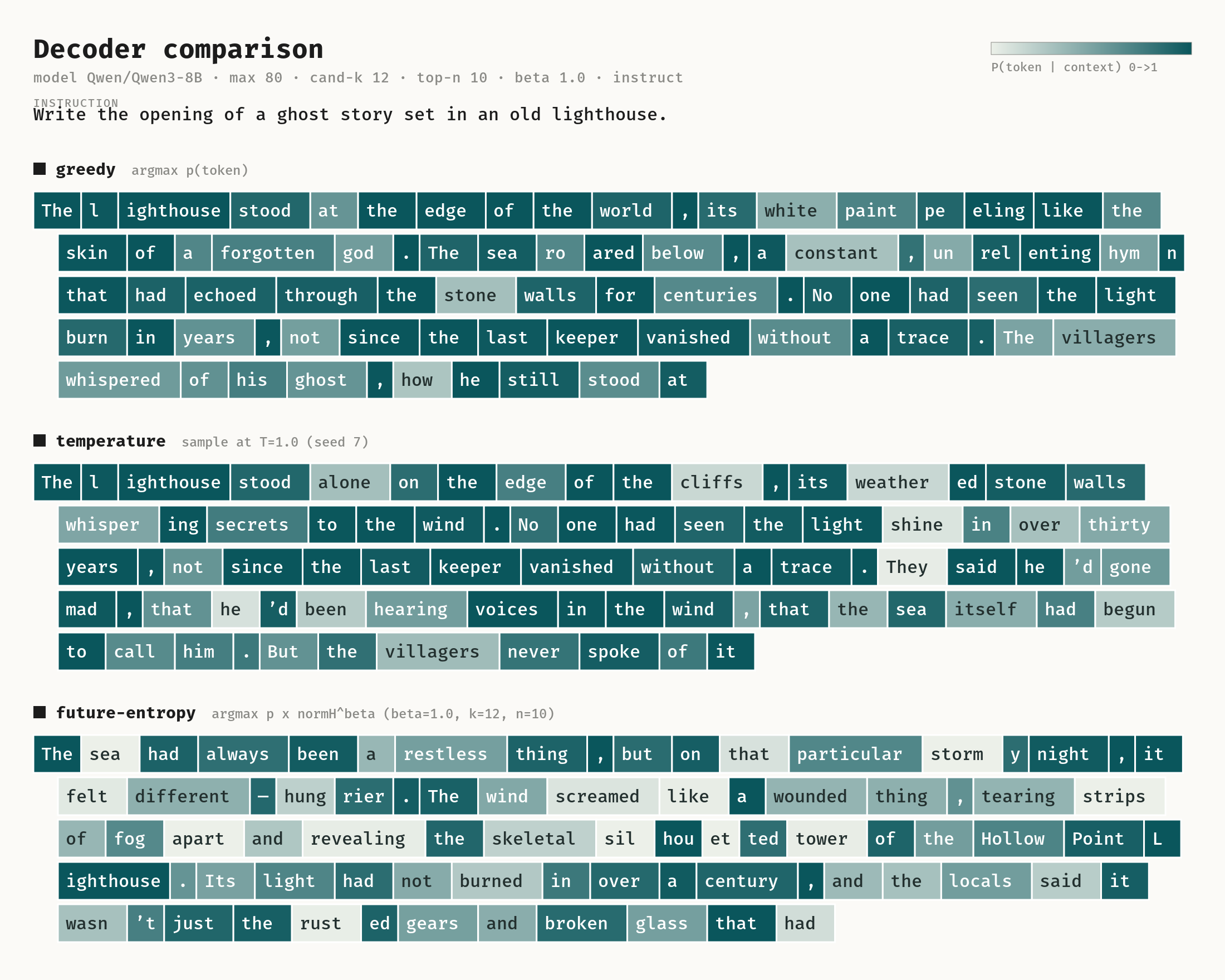
Comparing all three sampling approaches.

As you can see the first two samplers, including the “creative” temperature 1.0 sampler, choose results that are pretty typical LLM content. But our customer sampler produces results that, at least to me, feel quite refreshing and don’t necessary bear the typical hallmarks of AI writing.

With the base of our sampler figured out, let’s see if we can improve it a bit!

Generalizing our sampler - The α crossfader

Recall that our temperature based sampler used $T$ to generalize sampling from the token distribution, at one extreme it’s greedy and the other it’s uniform. We can perform a similar generalization by introducing a new parameter $\alpha$ between -1 and 1 that changes the balance in the scoring function between the original probability and the future entropy.

Mathematically this looks like:

$$s(w) = p(w \mid c)^{a} \cdot \hat{H}(w)^{b}, \qquad a = 1 - \max(0, \alpha), \quad b = 1 - \max(0, -\alpha)$$

Interestingly enough, when $\alpha = -1$, similar to when temperature is 0.0, our sampler reverts to being a much more like a traditional sampler. At the other extreme, $\alpha = 1$, the future entropy is the only factor (other than the fact that we’re constraining to the top n options).

In the image below we can see the results of this for the values -1, 0 and 1:

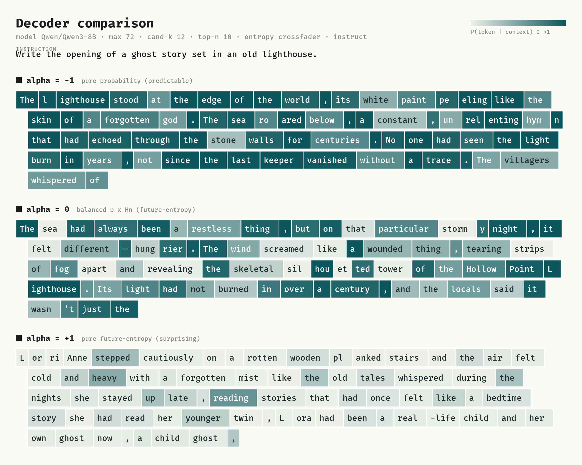
The first two results are pretty much what we had before and the third shows the impacts of pure entropy leading our path. Note that because we’re always choosing a path based on entropy, any individual token has a low probability.

Now which should we choose for our generation? Well, maybe we don’t have to choose!

Rhythmic decoding - the α-wave

For something approaching true creativity (and starting to feel like something earning the name ‘decoder’) why not mix up how we’re using our future-entropy sampler? Aside from aesthetics (0-2 as your temp!?) I chose -1 to 1 as the domain for $\alpha$ for a good reason: this maps nicely to the range of the sine function!

This means we can map a sine wave to our token generation process and use this to control our $\alpha$ allowing our writing to effectively breathe between different degrees of creative freedom. The intention here is to vary between predictable and unpredictable text creating even more engaging results. In the final image we can see the results of applying this technique:

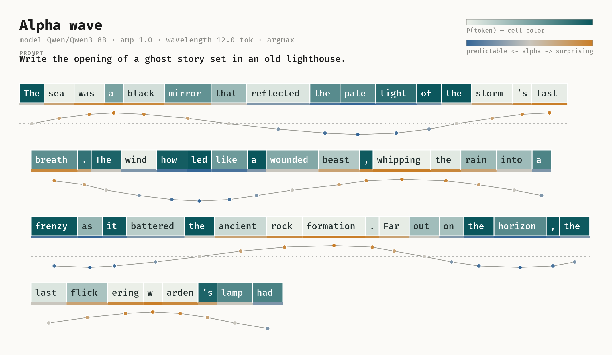
In this image we can see how $\alpha$ alternates between higher and lower values creating, imho, a much more compelling reading experience (especially for such a relatively small model!) This is probably the first time I’ve personally enjoyed reading the output of an LLM, and I definitely want to experiment more with reading longer versions of this output!

Conclusion

On the one hand, it’s easy to feel like LLMs are a bit overplayed at this point, on the other, I feel like we haven’t really started to explore what can be done with even the most basic aspects of the machinery behind these models! For awhile I had also held Ben Affleck’s view that LLMs simply aren’t going to be good writers, and I thought it was because of the fundamental nature of their architecture. Running this experiment has changed my mind a bit and made me curious about the ways we can apply more sophisticated sampling techniques to create much better creating writing from LLMs.

Want to explore more ways to be creative with AI!?

Then check out my book on AI image generation: Beyond Slop being released by in print by Manning soon! The basically complete version of this book is available in early access write now!