Inference and Prediction Part 2: Statistics
In part one of this series we built out a simple neural network (perceptron) to model the problem of Click Through Rate (CTR) for a job application website. At the end of our modeling process we realized the limitations of prediction and classification for solving a problem related to modeling CTR. The biggest insight we gained was that our real goal, to model a rate, was to understand a property of our model itself, rather than its output.
In this next part of our series we will focus on the problem of Inference which is commonly the domain of Statistics. When we perform inference we are much more concerned with the properties of our model itself rather than just its predictions. Since the goal of this series is to show the connection between machine learning and statistics, we will be continuing our example where we left off, building up all of the pieces of our statistical model from scratch.
Continuing with our Machine Learning model
As a quick refresher let's revisit the process we developed last time and see how this can directly lead us into a statistical model.
We began with a data set representing information about the users of a website who had viewed jobs and either applied or not. This is the list of features we have covering information about the similarity of various parts of the search with the posting, age of the posting and what category the job posting was in (we also have a constant for modeling purposes):
features
> ['main_query_tfidf',
 'query_jl_score',
 'query_title_score',
 'job_age_days',
 'job_16140',
 'job_31542',
 'job_41757',
 'job_42467',
 'job_45300',
 'job_51966',
 'job_67237',
 'job_69982',
 'job_77312',
 'job_82238',
 'job_other',
 'const']
These features are in a matrix, \(X\), and accompany a vector \(y\) of outcomes. Both of these were split into test and training data sets.
Our model was a perceptron which we can represent as:
$$y = g(Xw)$$
Were \(g\) is a non-linear function (we choose the logistic function) and \(w\) is a set of weights. In code the model looks like this:
prediction = logistic(jnp.dot(X_train,w))
We also explored how machine learning really is learning. To optimize our weights we used the negative log likelihood and gradient descent to find a value of our weights that optimizes how likely the data would be given our model. JAX was essential in the process for making it easy for us to compute derivatives. We'll be making use of these techniques again in this post.
Now we can pivot to thinking of this as a statistical problem
Inference - The Statistical World View
When relying on libraries and software packages we typically use different tools to perform Machine Learning and Statistics. For the ML work we did in the last post, useful packages to solve this might include scikit-learn or Keras, whereas for Statistical work we would use a library like statsmodels. While these tools are extremely helpful, they can obscure the connections between Statistics and Machine Learning. Writing these tools ourselves from scratch we can see how close they are. In fact, to continue on to modeling for statistics we can start exactly where we left off, we just need to change our perspective a bit.
The perceptron we built in part one is identical to Logistic Regression. When doing statistics we don't just view our features and weights as inputs to help us predict an output, but an actual model of how the world works. Here is an image that shows how we can re-imagine our perceptron from last time:
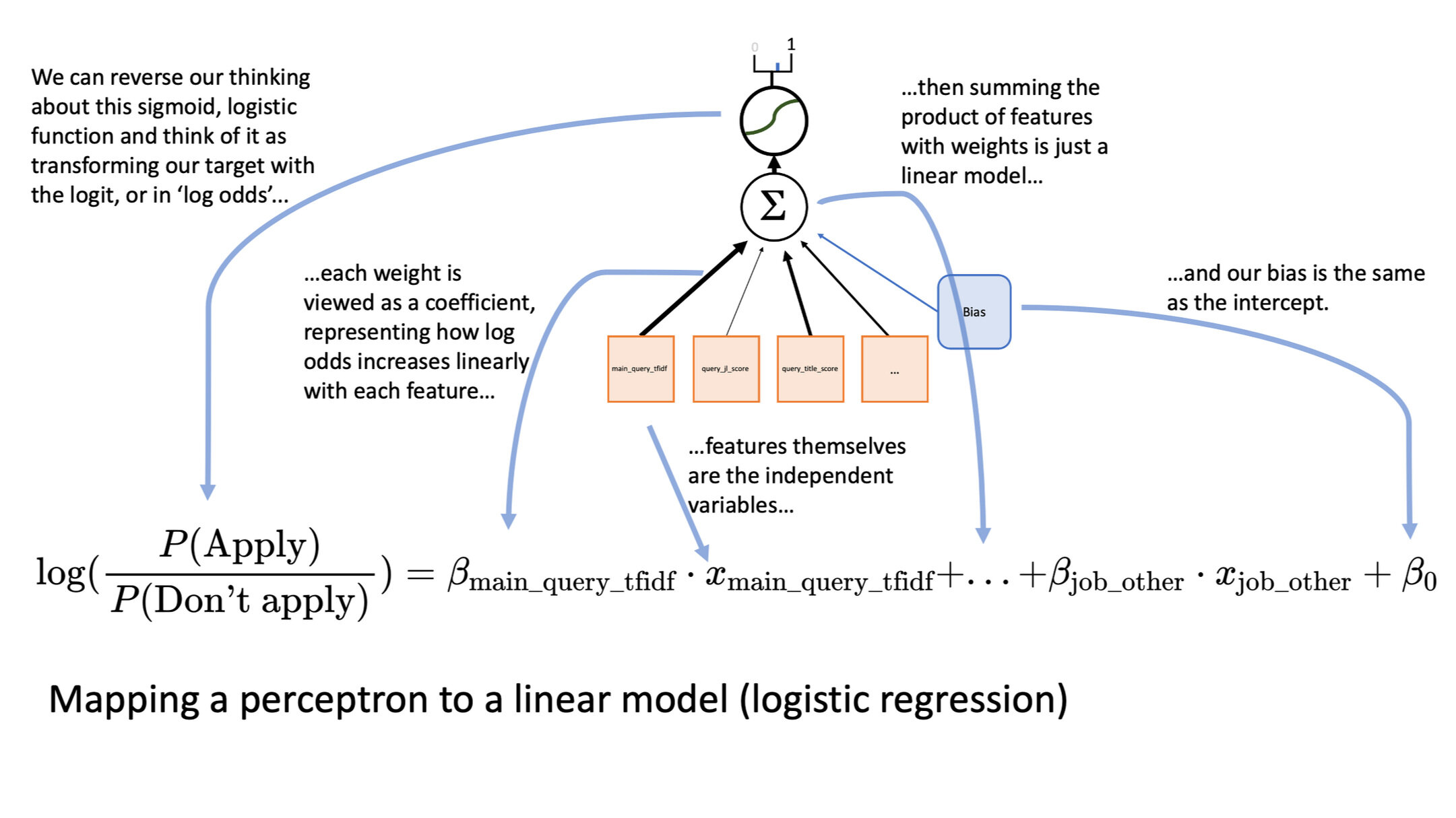
Even though the perceptron can feel quite different than logistic regression, our implementation is identical
In statistics we imagine each of the weights as a coefficient in our formula, and the bias unit from the perceptron becomes an intercept in a linear equation. The model says that each feature has a linear relationship with the log odds of a user applying for a job. If you would like a bit deeper of an insight, here is an earlier post for understanding the relationship between Bayes' Theorem and Logistic Regression.
This means that we are building a model to help us understand how each of the features might influence the probability of a user applying for a job on the website.
Inspecting and understanding our coefficients
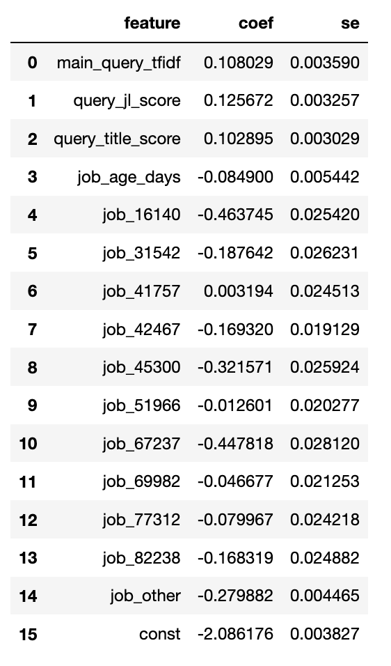
The very first thing we want to ask after training our model is “what did we learn about our coefficients?” We can put these in a data frame and start taking a look:
stats_df = pd.DataFrame()
stats_df['feature'] = features
stats_df['coef'] = w
Now we can take a look at we learned. These coefficients can be a bit tricky to understand since they are in log odds form, but we can play with these a bit to get a better intuition:

These values are in log-odds which can be tricky to interpret at first
As a general guide: positive values mean that as this feature increases so does the rate that the target event occurs. For example query_title_score represents how similar the job title is to the query string (the higher the more similar). We see that this coefficent is positive which means that the more similar the job title is to a user’s search, the more likely the user is to apply.
Right away we can see that this makes sense. If this value was negative it would be surprising and go against our intuition. This is one reason that, even when doing prediction, inference is essential. If this value was negative maybe we are wrong about how the world works... or maybe there's a bug in our code.
Negative values mean the opposite. The coefficient for job_ages_days is negative, which means that the older a posting is, the less likely a user is to apply.
Since we've mean centered most of our values (except the job categories) this means that the value at 0 is equivalent to the average behavior of this feature. This is helpful because it means we can ignore many of our coefficients when we want to compare values (we'll see this in a bit).
We have also normalized our values by dividing by the standard deviation, which means we can more or less judge the importance of a feature by the absolute magnitude of the coefficient. For example to offset the negative impact of being in job category job_16140, you would need to have a query_title_score roughly 4 standard deviations from the mean better than average!
Our intercept (‘const’ here), when all of our features are centered, become the log odds of the prior probability of a user applying (here's a whole post on prior probability in logistic regression). We haven't quite centered everything, but it's close enough to see this in action. We can use the logistic function to convert log odds back to probabilities. Let's take a look at what the prior probability should be in this model:
logistic(-2.086176)
> DeviceArray(0.11044773, dtype=float32)
You can see that it's not wildly different than the proportion of 1s in our training data (if we centered everything it would be even closer):
y_train.sum()/y_train.shape[0]
> DeviceArray(0.08990832, dtype=float32)
We can use this model to answer simple questions that might come up about the expected behavior of our job site. Suppose someone managing the accounts related to job_16140 came and asked you:
What rate should I tell clients they can expect people to apply?
We can estimate this very easily. Since all of our non-job category features area mean centered, on average they'll be zero so we can ignore them. The job categories are mutually exclusive so the only values in our model will be the intercept and 1 for job_16140. This means our answer is:
logistic(-0.463745 + -2.086176)
> DeviceArray(0.0724318, dtype=float32)
Now it's time to move on to the most important question of statistics: how sure are we?
Measuring our uncertainty
Each of the coefficients learned by our model is just a point estimate. We learned this by finding the set of weights that gave the most likely explanation of the outcomes given the data, but what if we had more data? And wouldn't a slightly different coefficient explain the data pretty plausibly?
In machine learning we view each of these estimates as a specific value, but in statistics we view them as the mean of a normal distribution of possible estimates. What we need now is to come up with the standard deviation of these distributions, in this case commonly referred to as the Standard Error.
Computing Standard Error from Negative Log Likelihood
There is a really fascinating connection between our objective function, the negative log likelihood, and the standard error. Recall that we found the optimal weights by using the first derivative of negative log likelihood to optimize. It turns out that we can use the second derivative of this function to determine how certain we are!
Since we used the negative log likelihood as our optimization function, it turns out that the square root of the inverse of the diagonal of the Hessian gives us the standard error of our coefficients. This is a lot to take in, so let's walk through it in code!
First we need to get the Hessian matrix, which is just a terrifying name for matrix representing the second partial derivatives of our function, which is itself a pretty scary way to say "how wide the curves are of our function in high dimensions". Aren't you glad we have JAX?
Here's an efficient JAX implementation to compute the Hessian efficiently:
from jax import jacfwd, jacrev
def hessian(f):
    return jacfwd(jacrev(f))
Now we need to get the Hessian at the point where we found the optimal weights, which is:
our_hessian = hessian(lambda w: neg_log_likelihood(y_train,X_train,w))(w)
our_hessian.shape
> (16, 16)
As you can see this is a 16 x 16 matrix representing the way each weight changes with respect to each other weight. For computing our standard errors, all we care about is the diagonal of this (because we are assuming each coefficient is independent of the others):
our_hessian_diag = jnp.diag(our_hessian)
The inverse of this give us our Variance...
coef_variance = 1/our_hessian_diag
And of course we wouldn't call it \(\sigma^2\) if we didn't really want our standard deviation, which is:
stats_df["se"] = jnp.sqrt(coef_variance)
Finally we can see how what our the standard error of our coefficients is:
That was a bit of work, but now all the rest of statistics falls out of this almost trivially!
And all the rest of statistics: z-scores, p-values, confidence intervals
After computing standard error a surprising amount to statistics can be derived from relatively simple transformations. We'll start by computing the z-score which is essentially how many standard deviations away from a normal distribution with a mean of 0 would our observed mean would be. This is very straight-forward to compute:
stats_df['z-score'] = stats_df['coef']/stats_df['se']
P-values measure the probability of being z-score standard deviations from the mean. We can calculate this easily as:
from jax.scipy.stats import norm
from jax import vmap
stats_df['p-value'] = 2.0*(1.0-vmap(norm.cdf)(
    jnp.array(stats_df['z-score'].abs())))
Personally I'm not a huge fan of p-values, but they can be pretty useful for quickly summarizing the results of our regression. What they confusingly tell us is "the probability that we got this result if the true value of the coefficient was exactly 0".
Much more useful is that we'd like to have the lower and upper bounds for out estimate for the 95% confidence interval. Here I'm using the term "confidence interval" to mean we are 95% sure the true value is somewhere between a lower and upper bound (lb and ub):
stats_df['lb'] = stats_df['coef'] - stats_df['se']*2
stats_df['ub'] = stats_df['coef'] + stats_df['se']*2
And now we have all of the basic results you would expect from a tool like statsmodels:

Here we have essentially replicated the results we would have gotten from a tool like statsmodels.
It is worth taking a moment to reflect how far we’ve come from the last post, while following a continuous flow of small tweaks to our initial work on the perceptron!
Hypothesis tests and parameter estimation
A surprising amount of important statistical information is contained in what we have learned about these coefficients. We can treat this information in slightly different ways to arrive at either a Frequentist or Bayesian perspective of our data. We can visualize all of these properties for the job_69982 coefficient:
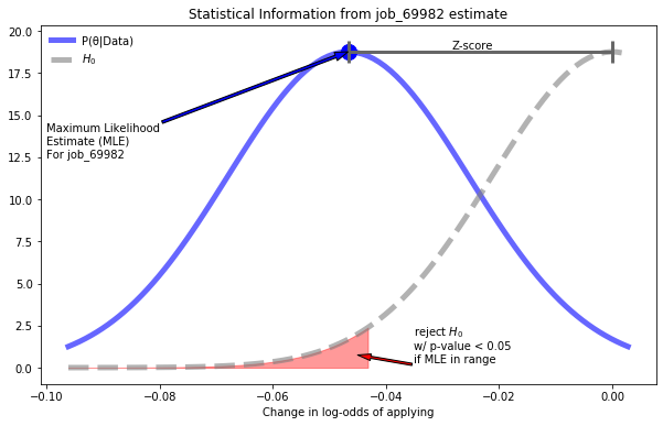
We can visualize everything we have learned about our weights
By understanding the various interpretations of the properties we see here we can use our model as a solid starting point for either Frequentist or Bayesian analysis.
Frequentist Hypothesis testing
From a Frequentist perspective the p-values of each coefficient tells us whether or not we should reject the null hypothesis, \(H_0\). In this particular case, the null hypothesis is that the coefficient is 0. In the specific case of job_69982 we can view the results here as an example of a Null-Hypothesis Significance Test (NHST), where we are testing whether or not job_69982 has an impact on a user applying. With a p-value of 0.028074 we would reject the null-hypothesis given the common significance threshold of 0.05.
If you've ever found Frequentist statistics tricky to wrap you head around, you're in for a happy surprise. Virtually every frequentist statistical test can be modeled as some variation on our linear model!
It only a slight exaggeration to say then, that in our continuation of our machine learning example we have essentially covered the majority of classical, Frequentist statistics.
Bayesian Parameter estimation
Bayesian's are much less concerned about whether or not the coefficient is zero, and instead focus on what we believe the value might actually be. That is, we are focused on parameter estimation. From a Bayesian perspective we view \(w\) as a vector of our parameters typically noted as \(\theta\). In Bayesian analysis we are always trying to solve our problem in terms of Bayes' Theorem:
$$P(\theta | \text{Data}) = \frac{P(\text{Data}|\theta)P(\theta)}{P(\text{Data})}$$
Note that \(P(\text{Data}|\theta)\) is the likelihood, which is directly related to our loss function. If we assume a uniform prior for $P(\theta)$ (something we can play with changing in part 3), then we can see that what our machine learning has also been learning is this exact model.
As Bayesians we are looking at \(P(\theta|\text{Data})\) as a distribution of beliefs, which in this model is really a Multivariate Normal distribution with the vector of means equal to \(w\) and the \(\Sigma\) a diagonal matrix corresponding to the se we learned. In this case we look at the lower and upper bound of each parameter as the limits of what we believe could be a realistic value for this parameter.
So our model provides a foundation for starting to understand our problem from both a Frequentist and a Bayesian perspective! Here we can see the wisdom of minimizing the negative log-likelihood since it allows us to connect machine learning with two different perspectives on statistics in a single model. Now we'll investigate how we can use all of this to start solving problems related to CTR.
Running Experiments
When modeling it is always important to keep our modeling efforts close to our actual goals. In this series of posts we've merely stated that the problem is to "model CTR", but to what end?
Presumably if we were a company that was listing job postings and we cared about the rate that applicants applied to postings we would want to increase that rate. Looking at our model helps us to think about how we would start to tackle this problem. By looking at our model we can see that we are very confident that "query_title_score" has a large impact on the rate that people apply.
This immediately leads us to thinking:
If there is a way we can increase the average similarity between the job title and the query, this should increase the apply rate
Which leads us to the next question "how can we do this?"
Always ask "what does this mean"?
But before tackling how we'll solve this problem it is vital that we always question what the model tells us about the world, and if we can form any coherent meaning around this.
As an example, once I worked at a company that tried to make less popular items sell better by moving them up higher in the search results. From a purely model based perspective this makes sense, items at better positions sell better. But it fails to answer questions about why items are in a better position in the first place: generally it's because they sell better. When we ran this experiment, with some exceptions, we generally found that items did not perform better (in some cases they performed worse!) when they were moved artificially to better positions.
So in our case we have to ask ourselves: why do we think a big difference between job title and query might occur, and do any of these cases present the opportunity to fix a genuine problem.
One case can be that someone searches "Data Scientist" and the result is "Accountant". Suppose this happens because "data entry" and "bachelor of science" are in the description. In this case the words are different and so are the meanings. If we somehow artificially changed the job title to match better we'll only frustrate the user.
However, another case is the user searches "Data Scientist" and "Associate Researcher (ML)" comes up. Assume that "Associate Researcher (ML)" is in fact essentially the same as a data scientist, but the user is confused and therefore doesn't apply.
Both of these scenarios are plausible, I personally think the first is more likely, but the real power of statistics is that we don't have to argue about what the impact is we can test it!
Testing a proposed solution
To solve this problem the Machine Learning team has come up with a clever natural language processing model that will rewrite job titles to have a higher probability of matching with semantically similar searches. This is great news, but the obvious question we need to ask is "does it really work?".
To test our title-rewriting model we decide to conduct a controlled experiment. We'll assign 20% of our users to a test group where the the titles in the result will be rewritten based on the query, and the rest will have the same experience as before.
After running the experiment for awhile we have a new set of data: X_exp and y_exp. These use the same setup as our original data with one new feature, representing whether or not the user was "in_test".
Now we can really see the beauty of models being interpreted as a sequence of hypotheses about the impact of the coefficient. Before building a model with our experiment data, we should first think about what we hope to see in the results.
Our goal is that users in our test group will apply at a higher rate then everyone else. So we want to see that our coefficient is positive. From the perspective of classical statistics, we want the p-value to be very small (even Bayesians can use this as a helpful heuristic). If this happens it means that we have strong evidence that our title rewriting logic worked!
To analyze our results we can build a new version of our model with the additional coefficients representing whether or not a user was in the test group. Notice that now that we've done all the work of creating our necessary functions, building this new model from scratch isn't too much work:
key = random.PRNGKey(123)
w_exp = random.uniform(key,
                       shape=(X_exp.shape[1],),
                       minval=-0.1,
                       maxval=0.1)

lr = 0.000001
for _ in range(1,300):
    w_exp -= lr*d_nll_wrt_w_c(y_exp,X_exp,w_exp)
print(neg_log_likelihood(y_exp,X_exp,w_exp))

> 257385.67
After repeating the process of building out stats data frame we have these results:

Looking at our test results it doesn’t look too good for our new rewriting tool
When we look at the results for in_test it looks like bad news. The coefficient is slightly negative (though only very slightly) but worst of all the p-value is large.
P-values don't tell us everything though, maybe just don't have enough data? We can get a clue for this by looking at the lower and upper bounds for our estimate. If these are large numbers it means there's a lot of uncertainty about what the value might really be, which means we don't really know. Unfortunately in this case these numbers are quite close to 0, which statistically means it looks like our clever title re-writer probably doesn't work...
...except we're missing a major piece of the modeling puzzle!
Causality
Here we see an object lesson in why it is so important for us to understand what we think will happen when we run our experiment. At the outset we declared that our title re-writer should increase the query_title_score, but we included the query_title_score in our model. Since the only impact, in theory, of the re-writer was to improve the query_title_score, controlling for this in our model will hide the impact that the test had!
That is there is a causal relationship between the test and the query_title_score, by observing the query_title_score in our model we remove any information we have captured about the test.
In order to solve this problem we need to rebuild a model that doesn't have the query_title_score.
Here is the code to do this:
key = random.PRNGKey(123)
X_exp_no_qs = jnp.array(np.delete(X_exp,2,axis=1))
w_exp_no_qs = random.uniform(key,
                       shape=(X_exp_no_qs.shape[1],),
                       minval=-0.1,
                       maxval=0.1)
We’ll skip over the code for the training since we’ve seen it a few times now and inspect what our in_test coefficient tells us now that we are correctly modeling causality:

Now that we are correctly modeling our problem we see the results are significant!
And now we see that in_test has a strongly positive value with an extremely low p-value. We are now pretty much certain that our re-writer is a success!
Our initial experiment model is not a waste though. If you know that a treatment should have an impact on one of the model coefficients, I always recommend seeing if including that feature can eliminate the test coefficient’s significance (or greatly reduce it). This is very helpful in debugging experiments. If we had included query_title_score and in_test was still significant then that would signal that there was something else, not controlled for in the model, that was causing our test group to perform better. I have had this happened in the past running experiments and it is a vital tool in correctly running tests.
Model Comparison with Akaike Information Criterion
Since we built two models in the last section, it's a good idea to take a moment to discuss how we compare models in statistics. In Machine Learning we are primarily concerned with the output of the model, so we come up with various metrics to compare the predictions of the model with the observed outcomes. In Statistics we are primarily concerned with the parameters and model complexity.
The common measurement for judging models in Statistics is some form of Information Criterion which balances the likelihood of the data given the model, with the model complexity. The most common is Akaike Information Criterion (AIC). In a case where \(k\) is the number of parameters in the model, and \(L\) is the likelihood, AIC is defined as:
$$\text{AIC} = 2k-2 ln(L)$$
Since we are using negative log likelihood, we would simply have:
$$\text{AIC} = 2k+2 \cdot \text{nll}$$
The absolute value of this metric doesn't matter, but in general a lower score is better when we compare models trained on the same data. Generally we want it to be the case that if we add parameters, we decrease AIC. We can see how our models did:
def aic(y,X,w):
    k = X.shape[1]-1 #because we have an interecept
    nll = neg_log_likelihood(y,X,w)
    return 2*k + 2*nll

aic(y_exp,X_exp,w_exp)
> 514803.34

aic(y_exp,X_exp_no_qs,w_exp_no_qs)
> 515627.5
We can see that adding the query score provides a much lower AIC. This means that adding just that one parameter to out model afforded us a much improved likelihood. The only reason we needed to remove this important feature was because it was impacting our ability to understand the results of our test.
Towards synthesis
A major limitation of statistical inference is that, traditionally, it tends to avoid computational thinking. Statistics, for most of its history is not a subject for hackers. Statistical software, like, statistical tests remained opaque and mysterious. Students of statistics may formally derive a closed from solution to the OLS version of regression, but after that its all up to some standardized software package. It's good to rely on abstraction, but without being able to build statistics from scratch there is little room to play, experiment and explore.
This is where Machine Learning, and in particular Deep Learning has really shined in the last decade. Watch any talk by experts in machine learning and you will encounter incredible playfulness. I still remember the excitement of watching Geoffrey Hinton's talks in 2012. Nearly all innovation coming out of deep learning comes from someone asking "what happens if we try this?"
Likewise building a neural network is no mystery for practitioners. Anyone seriously interested in neural networks and machine learning quickly has the experience of building one from scratch, then playing with that design to see what else they can do. Statisticians may criticize deep learning for its lack of rigor, and there is some value in the critique, but the lack of play in statistics remains perhaps its largest falling.
But now you have see how everything works in a statistical model, built from just basic math and linear algebra! In Part 3 we'll continue our exploration by applying the causal exploration the Machine Learning approach, with the attention to understanding our models that we get from the world of Statistical Inference. In truth there is no division between these two, just the delightful possibilities of mathematical exploration.

Support on Patreon
Support my writing on Patreon and gain access to the source code and video commentary for this article as well as access to much more of my writing!