The Logit-Normal: A ubiquitous but strange distribution!
Statistics is, at its heart, the study of how little you actually know about anything. Even for the beginner the first thing you learn is how much you don't know about the data you have. But it gets worse over time. Without a doubt, the more I study statistics the less I know I know about it. For example, 10 years ago I knew everything about logistic regression and today I know almost nothing about it all!
A wonderful object lesson in this is the logit-normal distribution. It seems innocuous at first glance: a logit-normal distributed random variable is one whose logit (log-odds) is normally distributed. Sounds straight forward enough, but here's an interesting piece of information: none of the logit-normal's moments have a analytical solution! This makes it a bit spookier than even the Cauchy distribution which has undefined moments. The logit-normal has them, we just can't find them exactly.
Adding to the mystery is that you have likely run into the logit-normal without recognizing it. If you've ever used logistic regression you have made tacit assumptions about this distribution, and they might very well be incorrect.
The Logit Function
As stated, a logit-normal distributed random variable is one whose logit is distributed normally. To make sense of this we need to review a few basic tools that we use very frequently when working with probabilities.
Recall that the logit is the log odds of a probability. So for starters we know that the logit-normal has the domain as a probability, being bound between 0 and 1 (technically a probability can be 0 and 1 exactly, where as the logit-normal is not defined for these extremes). The odds are the ratio of the probability of one event happening over an other, in the case of the logit, we are comparing the probability of an event happening, \(p\) to the probability of it not happening, \(1-p\).
$$o = \frac{p}{1-p}$$
For the log part of logit we just perform a log transform of our odds. So we can mathematically define logit as:
$$\text{logit}(p) = ln(\frac{p}{1-p})$$
The most common place we use the logit in statistics is in logistic regression since this allow us to take probabilities that are in the range \((0,1)\) and stretch them out so they become linear from \((-\infty,\infty)\). In our discussion of Logistic Regression from Bayes' Theorem we demonstrated how this allows us to learn probabilities with a linear model.
The Logistic Function
We're a step closer to being able to understand the logit-normal distribution, but we still need another valuable tool. We know that the distribution of a logit-normal random variable is a normal distribution. If we had a logit-normal random variable in our hand we could see that this was the case by transforming sample from that with the logit function and getting a normal distribution as the results. However what would be much nicer is if we could take a normally distributed random variable and see what logit-normal distribution it came from. For this we need the inverse logit or the more commonly named logistic function.
To derive the logistic function we just have to go backwards. Suppose we have an \(x\) that is the output of \(\text{logistic(p)}\) and we want to solve for \(p\). First we would have to raise \(e^x\) in order undo the fact that we took a log transform. This will leave us with the odds of the event happening. To transforming odds into a probability we can use the following formula:
$$p = \frac{o}{1+o}$$
We can put this all together to get:
$$\text{logistic}(x)= \frac{e^x}{1+e^x}$$
Which can be simplified as:
$$\text{logistic}(x)= \frac{1}{1+e^{-x}}$$
We're going to be using Python to play around with the logit-normal so we'll use these to helpful imports from scipy
import numpy as np
from scipy.special import logit
from scipy.special import expit as logistic
Sampling our Logit-Normal
As mentioned in the beginning, what makes the logit-normal really fascinating is that all of it's moments have no analytical solution! (Here is a post if you need a refresher on moments of a random variable. This means even expectation and variance are not easily discovered.
A good way to play with a logit-normal is to sample from a Normal distribution and then use the logistic function to transform those sample. We'll end up with a logit-normal because we know that applying logit to those transformed samples will get us back to our original normal distribution.
Let's start with the standard normal with a \(\mu=0\) and \(\sigma=1\).
Here we can see samples from this as well as the resulting logit normal:
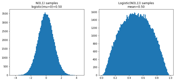
Samples from a standard normal and those samples transformed into a logit normal.
As we can see we have a very interesting distribution on the right here that stretches between nearly 0 and nearly 1. Since we generated this distribution by taking the logistic of the one samples on the left, if we take the logit of this distribution we will have our original Normal distribution.
I've added another important piece of information that, in this special case, can be very misleading. I've displayed both the logistic of the \(\mu\) parameter for the Normal, and the observed mean of the logistic of the samples. In this case they are identical.
However let's look at a normal distribution with a \(\mu=-5\) and \(\sigma=2.0\):

The logistic of the mean of the normal distribution is not necessarily the mean of the logit-normal corresponding to it.
First you'll notice we get a really interesting difference between the way these two distribution appear now. The most important thing to notice is that the logistic of the mean and the mean of the logistic samples are not the same!
This shouldn't be too surprising given that we know that the moments of the logit-normal have no analytical solution. If the logistic of \(\mu\) always equaled the mean of the logit-normal, then we would clearly have an easy analytical solution. It turns out that the logistic of the mean will give us the median of the logit-normal, which in many cases is quite useful, but the expectation of this random variable escapes us.
What makes this particularly interesting is that nearly everyone in statistics makes frequent use of the logit-normal distribution... and quite often we are doing so and ignoring this property of the logit-normal. I do it quite explicitly in part 2 of Inference and Prediction.
Interpreting Logistic Regression
Initially it might seem like the peculiarities of the logit-normal distribution are just a mathematical curiosity, with little impact on the practical things we do in statistics day-to-day. That is until you consider that Logistic Regression is learning parameter that are normally distribution in the logit space. That is interpreting the result of any logistic regression involves working with logit-normally distributed random variables. We'll explore this by looking at an example of a simulated A/B test that uses a Logistic Model as the foundation of our testing set up.
A/B Testing Example
For those unfamiliar, an A/B test is a common experiment in industry where we might have two variants of a web page (or really any part of the user experience) and we want to see which one performs better at converting the user according to a metric of interest (usually ‘clicks’). We've explored A/B Testing using the Beta distribution quite a bit, but we can also use logistic regression to perform an A/B test.
Our data is observations of clicks on a website (or purchase of product, signups on a webform, etc). The way we'll set this test up as linear model is:
$$\beta_\text{A}x + \beta_0$$
Where \(x\) is whether or not a subject was in experiment with variant A, \(\beta_0\) reflects the prior probability that a user will ‘click’, and \(\beta_A\) represents how being exposed to variant A changes that. Since we're estimating the probability of an event happeing we learn this using logistic regression where \(y\) indicates whether or not a user clicks:
$$y = \frac{1}{e^{-(\beta_\text{A}x + \beta_0)}}$$
We train a model on data and we'll find that \(\beta_\text{A} + \beta_0\) is the log odds estimate of the rate of A, and \(\beta_0\) on its own reflects what we think the log odds rate for B will be.
For our example we'll assume a case where both A and B have low probabilities of occurring. We'll simulate 5,000 observations of each. In these 5,000 observation of each we see the following number of successes
A - 28 successes
B - 32 successes
We then train a logistic model on this data and see what we learn. We can see the summary of our model here:
import statsmodels.api as sm

N = 5000

y_a = rs.binomial(1,a_true_rate,N)
y_b = rs.binomial(1,b_true_rate,N)
y = np.concatenate([y_a, y_b])

variant = np.concatenate([np.ones(y_a.shape[0]), np.zeros(y_b.shape[0])])

X = sm.add_constant(variant)
sm_model = sm.GLM(y,X,family=sm.families.Binomial()).fit()
sm_model.summary()

In this data const corresponds to our intercept \(\beta_0\) and x1 to the \(\beta_\text{A}\). Judging from this alone we can see that it looks like A might be the worse variant, but we aren't very confident in this result so far. The P>|z| part there gives us the p-value that we could use if we wanted to treat this as a standard null-hypothesis significance test. Clearly we don’t have enough data draw a conclusion, but for this exercise all we care about is the estimations we have for these parameters.
We're interested in what we expect for the rate for variant A to be. Since we're using statsmodels we can get our model to predict this for us.
We're going to create a simple vector representing the A variant, which consists of just an intercept and a 1 representing the variant, then use the predict method to calculate the models estimate:
sm_model.predict(a_vec)
> array([0.0056])
You'll notice that we could manually arrive at this result ourselves by taking the logistic of the sum of the parameters (that is \(\beta_\text{A} + \beta_0\).
logistic(sm_model.params.sum())
> 0.005600000000000602
Note: for those that are really interested in the details this is not exactly what statsmodels does, but it's close enough that it not does matter. You'll also get this same result if you use SKLearn instead (assuming you don’t use the default regularization).
Working with Normally Distributed Random Variables
As a quick refresher, let's take a moment to look at what's happening with our model when we think of it strictly as a linear model and ignore the fact that it is in logit space. For the case of A we have this equation:
$$\beta_\text{A}\cdot1 + \beta_0$$
What's important to realize is that in our case \(\beta_\text{A}\) and \(\beta_0\) are random variables. They represent estimations of the mean of these parameters. The coef value is the mean and the stderr value in the output is the standard error, or standard deviation of the estimate of mean.
So if we want to factor in all of our uncertainty and come up with a model we just follow the rules for adding random variables. Since our values of \(x\) are only 0 and 1 we can ignore the details of multiplying by a scaler. We can use following rule for adding normally distributed random variables:
$$X \sim \mathcal{N}(\mu_x,\sigma_x)$$
$$Y \sim \mathcal{N}(\mu_y,\sigma_y)$$
$$X+Y \sim \mathcal{N}(\mu_x + \mu_y, \sqrt{\sigma_x^2 + \sigma_y^2})$$
If we just need the expectation then all we need is sum the means:
$$E[X + Y] = E[X] + E[Y]$$
Hence, when we put all of this together adding \(\beta_\text{A} + \beta_0\) is giving us the mean of normal distribution representing our belief in the possible log odds for A. Then we just take the logistic of this value to come up with our estimate for the actual probability of A.
The true mean of our logit-normal
The issue here is fairly subtle. If we considered \(\beta_\text{A}\) and \(\beta_0\) as constants then it would be okay to simply take the logistic of these values... but what we have when we learn a model is that these values represent means of normal distributions.
As we know now we cannot trivially transform the mean of a normal distribution into the mean of its logit-normal shadow. In order to do that we need to user a bit of simulation. Here is the code that samples from the distribution of our estimate in the model parameters and then transforms those values with the logistic function, finally computing the mean of the true distribution these values represent:
logit_norm_mean = logistic(rs.normal(sm_model.params.sum(),
                     np.sqrt(np.sum(sm_model.bse**2)), 1000000)).mean()
logit_norm_mean
> 0.005876300819424593
As we can see, somewhat surprisingly, it is not the same! While in absolute value terms it's a small difference, this estimate is about 5% higher than the one we get form statsmodels!
The Beta Distribution
Readers of this blog, or the book might be quick to point out that while this difference in ways of interpreting the output of logistic regression is interesting, the more correct way to solve this this problem is to use the Beta distribution.
For a simple problem of estimating the rate of the A variant we don't need the complexity of learning a linear model (as simple as this may be), we can model our beliefs with a beta distribution.
For this case we'll want to use both a likelihood and a prior. For the likelihood we will define \(\alpha_\text{A}\) as the number of clicks and \(\beta_\text{A}\) as the number of non-clicks. For a prior we'll use \(Beta(1,1)\) which is our standard "non-informative" prior, stating very weakly that all rates are equally possible.
In order to compute the expectation of this distribution we use the following formula:
$$E[Beta(\alpha_\text{A}+1, \beta_\text{B} + 1)] = \frac{\alpha_\text{A}+1}{\alpha_\text{A}+1 +\beta_\text{B} + 1} = 0.0058$$
Which is remarkably close to the value we got out of our logit-normal simulation!
It turns out that while the logit-normal will never be exactly the same as a Beta distribution, the two can be remarkably close (close enough for any statistical purposes certainly!) The details are more than I want to dive into for this post but the Wikipedia has a pretty good discussion (just remember that the Dirichlet distribution is a generalization of the Beta).
What if we had no prior?
But that's not all! Proper Bayesian analysis requires us to use a prior distribution based on the fact that we're ultimately deriving our analysis from Bayes' Theorem. However if we look at just the likelihood, we'll find that the expectation it this case is... 0.0056! This is exactly the value we got out of statsmodels!
Conclusion: Towards Dionysian statistics
What do we do now? Which is the correct way to do things? If anything the greatest fault in statistical thinking is desperately trying to find the one concrete and correct way answer to these questions. Even I am guilty of this. It's a strange obsession for a discipline founded on meditation on how much we don't know.
Our world is in a state of collapse, though not everyone is as willing to admit it, in time it will become more and more clear. Even those not conscious of it can feel it in the air. In such a world I often wonder what is the future of statistics? I have found many statisticians I admire turn to statistics as a tool to hide from the realities of a rapidly changing world, clinging to thin strands of imagined certainty, and hiding doubt in complexity. But as our world changes the tools of statistics become harder and harder to use. The pandemic is a great example of this on a small scale. Everywhere models failed because models assume a static world. For larger problems, our models are not powerful enough to even comprehend the immediate peril we are in. So what good is statistics?
I was reading through Nietzsche's "The Birth of Tragedy" the other day, and came across an interesting analysis of Hamlet in light of what Nietzsche calls the "Dionysian man".
In this sense the Dionysian man resembles Hamlet: both have once looked truly into the essence of things, they have gained knowledge, and nausea inhibits action: for their action could not change anything in the eternal nature of things; they feel it to be ridiculous or humiliating that they should be asked to set right a world that is out of joint. Knowledge kills action; action requires veils of illusion: that is the doctrine of Hamlet, not that cheap wisdom of Jack the Dreamer who reflects too much and, as it were, from an excess of possibilities does not get around to action. Not reflection, no—true knowledge, an insight into the horrible truth, outweighs any motive for action, both in Hamlet and in the Dionysian man.
— Friedrich Nietzsche, The Birth of Tragedy
Nietzsche of course is thinking about the future of philosophy, but this got me thinking about what is the future of statistics. In Nietzsche's Dionysian/Apollonian dichotimy statistics would fall clearly in the realm of the Apollonian thinking: the rational, logical, certain understanding of what is. But when we stare deeply enough into small statistical problems, when we look at how little we understand about how little we understand, statistics becomes something quite different.
If there is a Dionysian statistics it is a statistics concerned only with uncovering how wrong we are and proving again and again how little we know. This is not to be confused with studying probability for probability’s sake, that is just the realm pure mathematics. What makes statistics distinct from pure probability its irresolvable friction with the world we are trying to understand. It is realizing that statistics is our only lens to understand the world, then poking at that lens until it starts crack under the pressure. Studying with fascination the cracks in the lens themselves, realizing whatever we hope to see on the other side will remain hopelessly distorted. Dionysian statistics is the act of dissolving the very truth it drives us uncover.

Support on Patreon
Support my writing on Patreon and gain access to the source code and video commentary for this article as well as access to much more of my writing!