People (well the tiny subset of them deeply and passionately interested in statistics) tend to argue a lot about the difference between "Bayesian" and "Frequentist" approaches to solving problems. Unfortunately these discussions remain largely at the level of trolling, memes and jokes (at least on Twitter), or, during moments of more enlightened discourse, entirely in the realm of philosophical speculation.

As much as I love a good speculative discourse, statistics is fundamentally an applied epistemology. Everything about this topic that's interesting comes out in praxis. It is much more interesting to look at actual examples of where Bayesian and Frequentist approaches disagree, see why they do, and try to understand the trade-off we are making when we choose one methodology over another.

The argument I am presenting here is that whenever there is a difference in the results between these two methods, it is always because the Frequentist approach is making shortcuts and is technically wrong. Very often being technically wrong means a minuscule difference in the result at a tremendous improvement in computation time. However ultimately it is important to recognize the trade-off rather than assume it.

We'll be taking a look at where these two schools of thought diverge in a specific case involving the endlessly fascinating problem of spinning coins. Or at least, something similar.

A simple problem: firing an Alien "slug" gun.

I do feel coins have been a bit abused, especially since you cannot intentionally bias a coin. A better tool for modeling really unknown scenarios is strange alien weapons, such as the slug gun depicted in an episode of Rick and Morty (pictured below):

Inter-dimensional travel presents some fun probability problems!

Suppose you stumble across this strange weapon and in attempting to get it to work you pull the “trigger” 9 times, and for all that effort get only 1 shot out. You want to know on your next pull of the trigger, what is the probability it will fire.

Here we have the classic probability problem of trying to estimate the rate that some event will happen in the future given that what we have observed about it happening in the past. We'll model this with a Bernoulli random variable:

$$X_\text{fires} \sim Bern(\theta)$$

What we want to do is model our beliefs in possible values for the rate of fire, $\theta$.

An Ad Hoc, frequently Frequentist, approach

Coming up with a point estimate for our rate is pretty straightforward and intuitive, $\frac{1}{9}$, but what we want to do is come up with a distribution of what we believe the true rate could be given the information we have.

If you discuss this with most people with some formal statistics training they will likely recognize this as a problem of computing the standard error of our mean. Thanks to the glory of the central limit theorem we can safely assume that means of random variables are Normally distributed. We already know our $mu=\frac{1}{9}$, but now we need to determine the standard deviation of our distribution.

To solve this, we will use another standard formula, sometimes refereed to as the Standard Error of a Proportion:

$$\text{SE}_\text{proportion} = \sqrt{\frac{p(1-p)}{n}}$$

If this formula is unfamiliar to you, don't worry, it was for me for a long time as well since I went through the path of Bayesian statistics first. For others this formula will be so familiar that it's existence will seem obvious, a bit too obvious if you ask me. I have found this is a pretty common pattern in Frequentist statistics: either you have memorized a bunch of rules that you don't quite remember where they came from, or everything seems to be a bit of a confusing mystery, with lots of unanswered "whys".

What we have here is a classic Frequentist Ad Hocism which combines a few common tools in a way that is seemingly rigorous, but classically confused about what it is actually trying to accomplish. This formula is born out of two important, well understood mathematical tools.

Standard Error

The first is the standard error, which is the standard deviation of the estimate of the mean for observations $x$ being sampled from a distribution:

$$\sigma_{\bar{x}} = \sqrt{\frac{\sigma^2}{n}}$$

Here the plain $\sigma^2$ is the variance of our observations of $x$, and $n$ is just the total number of observations. If we are assuming that we are working with purely random variables, we can derive this formula in a relatively straightforward way.

This little formula is foundational to a large part of Frequentist testing frameworks. It's important because it leverages the fact from the Central Limit Theorem that the mean of random variables will be normally distributed. This formula helps us fully represent our uncertainty in the mean. While this formula is quite sound for the case of pure mathematical objects, there is a surprising amount of hidden complexity in this when working with real data, but I’ll save that discussion for another post.

Variance of a Bernoulli Random Variable.

So given the standard error we next need to figure out what $\sigma^2$ is for our data. Since we are modeling our samples as a Bernoulli random variable we can just use the variance for that which is defined as:

$$Var[\text{Bern}(p)] = p(1-p)$$

Where $p$ is the probability of success. Putting those two together it looks like we have a great answer for our problem... and we sort of do.

But let's look and think about what we have here.

For starters we're not really answering our question. What we want is a distribution of what we believe the rate of fire could be. What Frequentist methods are attempting to do is come up a distribution representing the error around the mean of our estimate. So philosophically we’re setting out for different task depending on which school of thought you come from. In this case, this philosophical distinction shouldn't be a big deal since the "rate" is really just the expected ratio of fires to failures. It’s a bit of a happy coincidence that the Bayesian posterior and Frequentist standard error of mean, mean pretty much the same thing here.

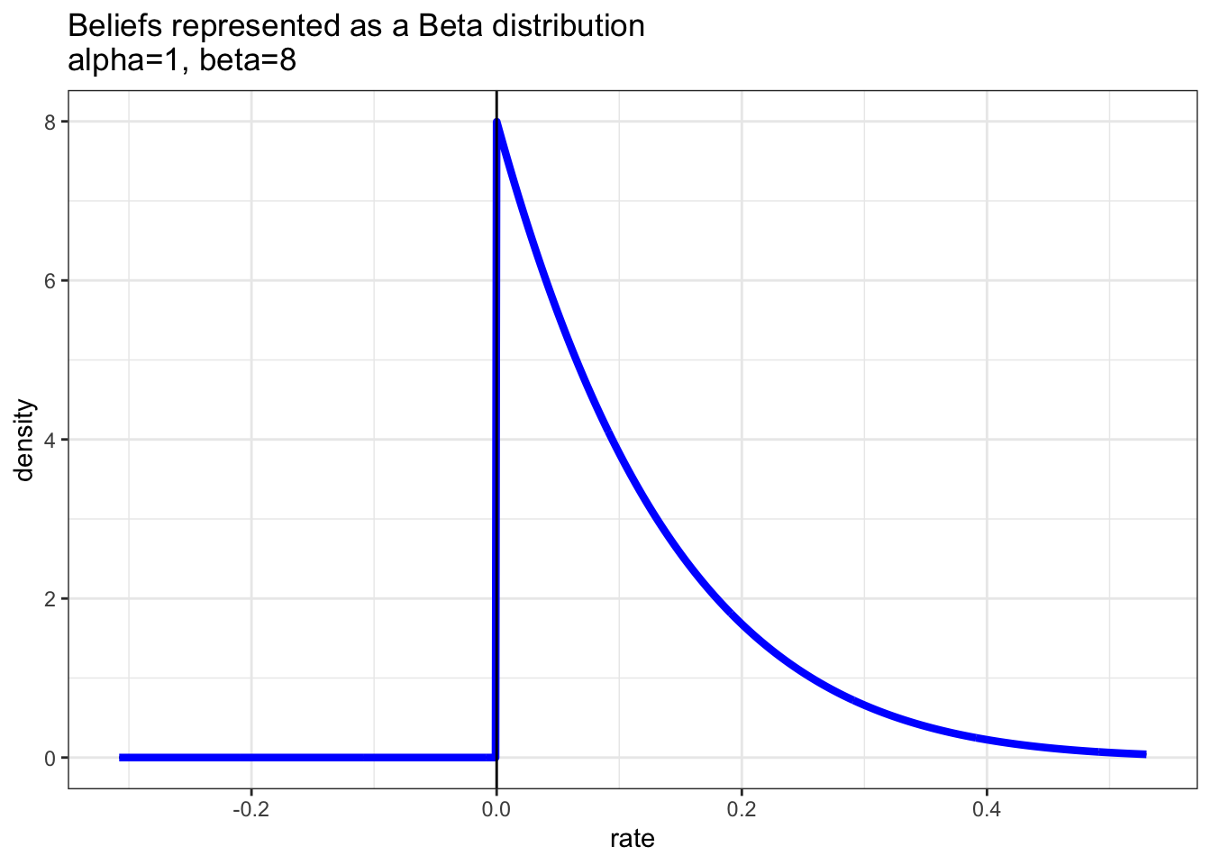
So this approach should yield what we want. When we plot out the distribution of our beliefs, we see it looks like this:

When we plot out these beliefs we find they are impossible

Yikes! It looks like a pretty large mass of our beliefs are... impossible!

Ad Hocisms

This doesn't work in this case because it is, technically wrong. The method we used to derive our Standard Error of the Proportion is what E.T. Jaynes would refer to as an Ad Hocism. We didn't derive this formula from probability theory properly, but rather by throwing together a few mathematical tools that look right together in an ad hoc manner.

If you have ever found Frequentist statistics to be confusing, this is why: because Frequentist statistics frequently skirt mathematics for ad hoc rules such as this one. Individually Standard Error is mathematically sound, as is the variance of a Bernoulli random variable. However slapping them together to make our standard error of a proportion doesn't quite work in all cases. What we’ve done is quietly made a normal approximation of something… without even answering the question of what we are approximating.

As we will see in a bit, somewhat surprisingly, that's actually okay nearly all of the time.

Now before any Frequentists jump at me screaming about formulas with names involving Wilson and Pearson, there are a fairly large number of ways to try to understand this problem better in a Frequentist framework. But pointing to a catalog of techniques and saying "one of those does better!" only further demonstrates the problem of ad hocism. Without a clear, logically and mathematically consistent framework for building out statistical tools, you end up with a catalog of tricks that don't always work like you would expect, and nobody quite knows all the edge cases.

The correct and, coincidentally, Bayesian approach

Because I took a rather strange path to statistics, I came across the Frequentist method for estimating beliefs in Bernoulli distributed random variables a bit later in my statistics journey. When I first was presented with the problem of estimating a Bernoulli random variable, before I even knew I was a Bayesian, tried to figure out how to solve this problem using the tools of probability.

My route of thinking was:

- We can view our Bernoulli r.v. and trials, as a single case of a Binomial r.v. and look at the probability of 1 success in 9 trials (the $\theta$ will be the same for either case)

- Then we consider all possible Binomial distributions that could have generated the data we have

- Finally normalize those so that they become a probability distribution

A bit more insight into this can be found in this post on probability distributions. After hacking around with some solutions and researching, I found this approach leads to the Conjugate Prior for a Bernoulli/Binomial distributed random variable: the Beta Distribution.

Given that the Beta distribution is by far the most used distribution on this blog I won't spend much time going over it. You can read up on parameter estimation, Beta priors, and hypothesis testing with Beta distributions at various places on this blog.

The Beta distribution is the mathematically correct (well not quite, we are still missing our prior) way to model the fact that we have seen 1 success, the $\alpha$ parameter, and 8 failures, the $\beta$ parameter. We also get a different formula for our variance the Beta distribution, our Variance is defined as:

$$Var[\text{Beta}(\alpha,\beta)]=\frac{\alpha \beta}{(\alpha + \beta)^2 (\alpha + \beta + 1)}$$

If we wanted to an equivalent to our Standard Error from earlier we would just take the square root of this.

This is not the variance of a normal distribution but of course the variance of a Beta distribution. When we plot out our beliefs we see a very different shape than earlier.

There are no impossible values now that we are representing this correctly

Here we have a correct method for modeling the likelihood of our beliefs given the data we observed. Notice impossible values are not represented here.

Many ways to be technically correct

There is no argument in favor of the "Standard Error of a Proportion" being correct for this specific problem, we can see in this example that assuming a normal distribution clearly gives us an impossible representation of our beliefs.

However, just because our Beta distribution estimation is the technically correct approach, doesn't mean we have no room to argue with this model in alternatively correct ways.

For example, something seems quite wrong with this to me because so much density is near 0. An experienced Bayesian will recognize that this is because this is just a likelihood function in a vaccum, and Bayes’ theorem will demand that we have a prior to truly represent our beliefs correctly. Again, this isn’t a trick that feels good, or merely looks correct. We can formally derive all the inference rules we need through mathematical reasoning with just the sum and product rule of probability.

In this case adding the Beta(1,1) prior (aka the Laplace Prior), meaning we weakly believe that all rates are equally likely, we can modify this result:

The correct representation of our beliefs given the information we have.

What we have here is a technically correct and perfectly justifiable answer to the question "What do we believe about the rate the slug gun fires?"

We could easily argue about a range of different choices in priors etc, but the important thing to observe here is that within the space of mathematically correct reasoning, there is room for nuance.

Alternative but equally correct solutions aren't limited to adding priors either. Maybe you don't believe that a Bernoulli random variable is a good representation of our process. Perhaps you believe that, as we get more familiar with the weapon, our rate of fire will improve. There are an infinite variety of mathematically correct ways to model this problem. All you need to do to expand is to come up with the correct representation of the probability of your data given your model, prior probability for your model and some way to normalize it correctly into a probability distribution.

But aren't Priors just an "ad hocism"!?

I've had to skim over a lot of theory in this post, but a very reasonable question someone without much experience in Bayesian methods might ask is whether or not the prior is just as ad hoc as the standard error of a proportion.

Whenever we have a problem where we struggle to come up with a prior it is because we lack information about the problem at hand. For example if you think that Beta(99,1) is a more correct prior, you and I will get very different answers to the behavior of this gun.

But this doesn't mean that our framework for inference is ad hoc. The fact that you and I having different prior beliefs leads to different results for very logical and clear reasons is evidence for how consistent our framework is.

If different priors give different results, and we don't know which prior is better, then we need to learn more about our problem. No amount of mathematical rigor will help us if we don’t have enough information. Neither will pretending we don't have this problem by hiding it in the ad hoc mechanics of our inference framework.

An important defense of Bayesian methods

Here I do want to make a point that Bayesians are frequently shy about: there's nothing "Bayesian" about this approach, using the Beta distribution is the mathematically correct way to solve this problem. The Bayesian and Frequentist methods do not represent two equally valid, mathematical points of view on the problem. The Bayesian approaches are literally just the basic rules of probability correctly applied to perform inference. Whenever Frequentist and Bayesian methods differ, it is because Frequentist methods are resorting to an ad hoc technique, rather than using mathematical reasoning to solve the problem correctly.

Misunderstanding this can lead to some confusion about when Bayesian and Frequentist approaches differ. Take this tweet from Daniël Lakens which coincidentally came up while I was in the middle for drafting this post:

"The main difference between a frequentist and Bayesian analysis is that for the latter approach you first need to wait 24 hours for the results."

This is a critique of the fact that Bayesian methods can be computationally expensive to run, often for the same result. It is true that Bayesian methods can be more expensive to run. However Frequentist approaches would be just as expensive if they were using equally as rigorous methods. The reason the Frequentist methods can seem faster is because ad hoc rules and short cuts are baked deep within the system of frequentist reasoning.

It's worth mentioning that Allen Downey has a great post up now looking at this issue from different, but well worth reading, perspective.

If you had never heard of statistics, but had the full computational and mathematical tools we have today, you would, following the correct rules of mathematics, come to the Bayesian conclusion for the best estimate of the distribution of our beliefs given the observations we saw, even if you had never heard of Bayesian statistics.

This is exemplified by the fact that a huge number of guests on Alex Andorra's incredible Learning Bayesian Statistics podcast come from non-statistical backgrounds (myself included). These are largely people that have strong quantitative and computational backgrounds, but needed to discover statistics on their own. From that perspective Bayesian statistics is just the logical path of applying technical expertise to the problem of inference.

Frequently, being a little wrong is quick, easy and just fine

If you're expecting a rant about how we must abandon Frequentist methods for Bayesian ones in the name of mathematical justice... you won't find one here! (but if you do want that, I highly recommend spending some time with Michael Betancourt’s writing on the subject).

It turns out that despite spending a huge amount of my time thinking, writing and talking about Bayesian methods, I use Frequentist methods... frequently! In fact I shipped some code that made use of the standard error of a proportion just recently (which is what got me thinking about this problem in the first place). Is it because I don't care at all about truth and justice? No! It's because these methods did evolve for a reason: in a world of limited computational resources, where even integrating a normal distribution took time, these methods were fast and in most cases close enough.

I really can't stress enough that in any case where Frequensist methods differ from Bayesian methods Frequentist methods are technically wrong. But, it's important to ask "how wrong?" and see if that matters all that much. Even in Bayesian methods we need to rely on imperfect solutions such as using Monte Carlo simulations for integration. And sometimes mathematically correct is just not feasible.

Clearly in the case of 1 fire in 9 tries we can see that the Frequentist approach gives us a non-sense distribution of our beliefs. This is primarily an artifact of $\alpha + \beta$ being very small. But what happens as $\alpha + \beta$ grow? Normal approximations, even though they are on the range of $(-\infty,\infty)$, are often useful because when the variance is reasonably small, theoretically impossible values become practically impossible as well and so there is no issue. To see how this problem gets resolved we can compare the difference in variance between these two solutions.

Comparing Variances

Here is our problem in more detail. The variance (not standard deviation) of our normal approximation according to our calculation is:

$$\frac{p(1-p)}{n}$$

But the variance for the Beta distribution is:

$$\frac{\alpha \beta}{(\alpha + \beta)^2 (\alpha + \beta + 1)}$$

Even if we were going to approximate our Beta distribution with a Normal, it would make sense to parameterize the Normal with the same variance as the Beta distribution. But here we seem to have two different definitions of what that variance is.

To start with it's not even entirely clear that these aren't the same. We can make this more obvious by rewriting our standard error variance in terms of $\alpha$ and $\beta$ given these identities:

$$n = \alpha + \beta$$

$$p= \frac{\alpha}{\alpha + \beta}$$

With these we can see that our equations are, in fact, not the same:

$$\frac{p(1-p)}{n}= \frac{\frac{\alpha}{\alpha + \beta}(1-\frac{\alpha}{\alpha + \beta})}{\alpha + \beta}$$

And we can establish that:

$$\frac{\frac{\alpha}{\alpha + \beta}(1-\frac{\alpha}{\alpha + \beta})}{\alpha + \beta} \neq \frac{\alpha \beta}{(\alpha + \beta)^2 (\alpha + \beta + 1)}$$

But what is the difference? Well, thanks to the magic of Wolframalpha we can see that the difference of these two is:

$$\frac{\frac{\alpha}{\alpha + \beta} (1-\frac{\alpha}{\alpha + \beta})}{\alpha + \beta} - \frac{\alpha \beta}{(\alpha + \beta)^2 (\alpha + \beta + 1)}=\frac{\alpha \beta}{(\alpha + \beta)^3 (\alpha + \beta + 1)}$$

Just by looking at the denominator of the solution we can tell that this will quickly mean less and less as the sum of $\alpha + \beta$ grows.

For the simple case of $\alpha = \beta$ we can visualize this trend in the difference:

Very quickly the difference between “technically wrong” and not disappears.

As we can see in this chart, while the two methods of calculating variance will never be exactly the same, the difference quickly drops to nearly zero.

This is a common pattern in Frequentist methods since they also tend to make heavy use of asymptotic assumptions. Often, as we go to infinity the difference between methods tends to disappear. However, I spend very little time anywhere near infinity so I find it good to be careful about these assumptions.

Conclusion

In this case there will be no practical difference in performance between the Bayesian and Frequentist methods on modern computers. However, if we were to build out increasingly more complex usage of these tools we would find that Bayesian methods do start becoming more computationally intensive.

The key is to see the reason for this difference: doing things correctly is hard and expensive. Anyone who has studied numerical methods will know that engineering numeric solutions requires a range of trade-offs for efficiency.

Given all that, I still find Daniël Lakens’ message quite dangerous at face value. Whenever Frequentist methods give you a speed boost it is because they are taking a Mathematical short cut. But the foundation of your statistical inference being taking efficient short cuts means that you never really know which risks you're taking and when you are taking them as you build complexity into your models and inference. This leads to magical thinking where ad hocism replaces probabilistic reasoning. I don't think it's unfair to attribute part of the reproducibility crisis to reducing statistics to a bunch of fast, but ultimately poorly understood tools.

There is nothing that prevents a good Bayesian from also choosing to take short cuts. For example I will frequently use a vanilla implementation of the Generalize Linear Model, because for many problems I work with, I'm comfortably assuming a Beta(1,1) prior and taking the Laplace approximation for my uncertainty. As mentioned earlier, I shipped some statistical tests that used the standard error of a proportion. But in each of these cases these decisions were engineering choices, where I understood the risks, checked for places where this could get me in trouble and chose the tradeoff.

Support on Patreon

Support my writing on Patreon and gain access to the source code and video commentary for this article as well as access to much more of my writing!